(论文)[EGSR-2014] Probabilistic visibility evaluation using geometry proxies
Probabilistic visibility evaluation using geometry proxies
- Stochastic Visibility Evaluation 的续作,感觉跟近几年有偏转无偏的方法有些像
- 论文在求 visibility 的时候,因为直接求交太慢,因此使用 proxy 几何进行求交
- 此外使用随机采样的方式进行修正
- 实验结果证明能够支持更多的 shadow ray 求交【半影区域特别多的情况不行】,但是 MSE 变高了,说明引入的噪声更严重;只是一种实验性的思路
理论框架
- \(x,y\) 之间有很多几何原体 \(\mathcal{P}=\{p_1,p_2,\cdots,p_n\}\)
- 可见性【有一个不可见,那就是不可见】【一个为 0,就是全为 0】
\[ V_{\mathcal{P}}(x,y) = V_{p_1}(x,y)\cdot V_{p_2}(x,y)\cdots V_{p_n}(x,y) \]
- 可以通过一个代理 \(\mathcal{P'}=\{p_1',p_2',\cdots,p_n'\}\)
近似计算
- 通过近似提高效率
- 差异越大,误差越大
\[ V_{\mathcal{P'}}(x,y) = V_{p_1'}(x,y)\cdot V_{p_2'}(x,y)\cdots V_{p_n'}(x,y) \]
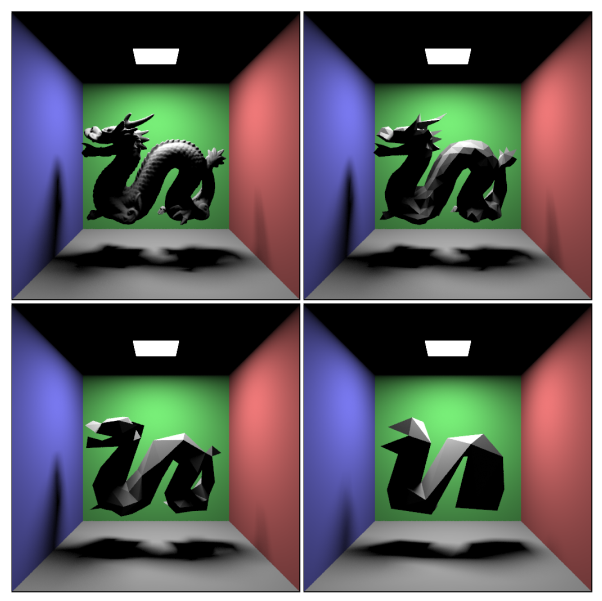
- 完整的可见性,可以进行修正
\[ V_{\mathcal{P}}(x,y)=V_{\mathcal{P'}}(x,y)+c(x,y) \]
- 分为 4 类光线
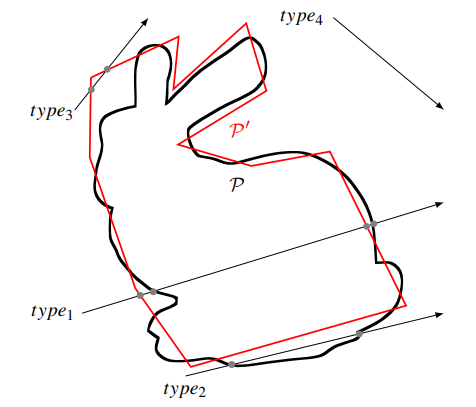
| Ray type | \(V_{\mathcal{P}}(x,y)\) | \(V_{\mathcal{P}'}(x,y)\) | \(c(x,y)\) |
|---|---|---|---|
| type 1 | \(0\) | \(0\) | \(0\) |
| type 2 (under-occlusion) |
\(0\) | \(1\) | \(-1\) |
| type 3 (over-occlusion) |
\(1\) | \(0\) | \(1\) |
| type 4 | \(1\) | \(1\) | \(0\) |
- 二值表,得到展开结果
- \(\bar{a}=1-a\)
\[ V_{\mathcal{P}}(x,y)=V_{\mathcal{P}'}(x,y)+V_{\mathcal{P}}(x,y)\overline{V_{\mathcal{P}'}(x,y)}-V_{\mathcal{P}'}(x,y)\overline{V_{\mathcal{P}}(x,y)} \]
随机估计
- 和前作 Stochastic Visibility Evaluation 一样,引入随机估计【保持无偏】
- 每一项 pdf \(p_i\)
| Ray type | \(V_{\mathcal{P}}\) | \(V_{\mathcal{P}'}\) | \(\dfrac{V_{\mathcal{P}'}}{p_1}\) | \(\dfrac{V_{\mathcal{P}}\overline{V_{\mathcal{P}'}}}{p_2}\) | \(-\dfrac{V_{\mathcal{P}'}\overline{V_{\mathcal{P}}}}{p_3}\) |
|---|---|---|---|---|---|
| type 1 | \(0\) | \(0\) | \(0\) | \(0\) | \(0\) |
| type 2 | \(0\) | \(1\) | \(\dfrac{1}{p_1}\) | \(0\) | \(-\dfrac{1}{p_3}\) |
| type 3 | \(1\) | \(0\) | \(0\) | \(\dfrac{1}{p_2}\) | \(0\) |
| type 4 | \(1\) | \(1\) | \(\dfrac{1}{p_1}\) | \(0\) | \(0\) |
方差分析
- 定义 \(f_i\):考虑所有光线 \(\overline{xy}\),,属于类别 \(i\) 的比例
- 此时平均 visibility \(V_{avg}=f_3+f_4\)
- 考虑 \(\mathcal{P}'\)【如下两个是一致的情况】
\[ f_{hit}=\frac{f_1}{f_1+f_2}, \quad f_{miss}=\frac{f_4}{f_3+f_4} \]
- 不同情况的方差:认为平均可见性 \(V_{avg}\)
- 这里为什么不和前作一样,考虑每一类自己的均值呢?为了分析全局方差?
| Ray type | Fraction | Variance |
|---|---|---|
| type 1 | \(f_1\) | \(0-V_{\mathrm{avg}}^2\) |
| type 2 | \(f_2\) | \(\dfrac{1}{p_1}+\dfrac{1}{p_3}-V_{\mathrm{avg}}^2\) |
| type 3 | \(f_3\) | \(\dfrac{1}{p_2}-V_{\mathrm{avg}}^2\) |
| type 4 | \(f_4\) | \(\dfrac{1}{p_1}-V_{\mathrm{avg}}^2\) |
- 全局方差
\[ \operatorname{Var}\!\left[\widetilde{V}(x,y)\right] = \mathbb{E}\!\left[\widetilde{V}(x,y)^2\right] - V_{\mathrm{avg}}^2 = f_2\left(\frac{1}{p_1}+\frac{1}{p_3}\right) + \frac{f_3}{p_2} + \frac{f_4}{p_1} - V_{\mathrm{avg}}^2 \]
\[ \begin{aligned} \operatorname{Var}\!\left[\widetilde{V}(x,y)\right] &= \mathbb{E}\!\left[\widetilde{V}(x,y)^2\right] - V_{\mathrm{avg}}^2\\ &= \frac{ \left(1-V_{\mathrm{avg}}\right) \left(1-f_{\mathrm{hit}}\right) \left(p_1+p_3\right) }{ p_1p_3 } + \frac{ V_{\mathrm{avg}}\left(1-f_{\mathrm{miss}}\right) }{ p_2 } + \frac{ V_{\mathrm{avg}}f_{\mathrm{miss}} }{ p_1 } - V_{\mathrm{avg}}^2 \end{aligned} \]
Outside proxies
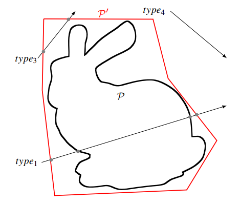
- 此时 type 2 不存在
- 即 \(\mathcal{P}\) 有交点,则 \(\mathcal{P}'\) 一定有交点
- 简化
\[ V_{\mathcal{P}}(x,y) = V_{\mathcal{P}'}(x,y) +V_{\mathcal{P}}(x,y)\overline{V_{\mathcal{P}'}(x,y)} \]
\[ \operatorname{Var}\!\left[\widetilde{V}(x,y)\right] = \frac{ V_{\mathrm{avg}}\left(1-f_{\mathrm{miss}}\right) }{ p_2 } + \frac{ V_{\mathrm{avg}}f_{\mathrm{miss}} }{ p_1 } - V_{\mathrm{avg}}^2 \]
Inside proxies
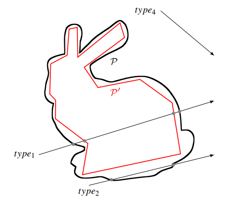
- 要求 \(\mathcal{P}\) 水密
- 此时 type 3 不存在
- 即 \(\mathcal{P}\) 没有交点,则 \(\mathcal{P}'\) 一定没有交点
- 简化:\(f_{miss}=1\),\(p_2=0,p_1+p_3=1\)
\[ V_{\mathcal{P}}(x,y)=V_{\mathcal{P}'}(x,y)-V_{\mathcal{P}'}(x,y)\overline{V_{\mathcal{P}}(x,y)} \]
\[ \operatorname{Var}\!\left[\widetilde{V}(x,y)\right] = \frac{ \left(1-V_{\mathrm{avg}}\right) \left(1-f_{\mathrm{hit}}\right) }{ p_1(1-p_1) } + \frac{ V_{\mathrm{avg}} }{ p_1 } - V_{\mathrm{avg}}^2 \]
实际算法
- 确定 \(p_i\),求导最小化
最小化方差
Inside proxies
\[ p_1 = \frac{1-f_{\mathrm{hit}}\left(1-V_{\mathrm{avg}}\right)}{V_{\mathrm{avg}}} - \frac{ \sqrt{ \left(1-f_{\mathrm{hit}}\right) \left(1-V_{\mathrm{avg}}\right) \left(1-f_{\mathrm{hit}}\left(1-V_{\mathrm{avg}}\right)\right) } }{ V_{\mathrm{avg}} } \]
- \(p_2=0\)【不存在这种情况】
- \(p_3=1-p_1\)
Outside proxies
- \(p_3=0\)
- \(p_2=1-p_1\)
\[ p_1 = \frac{ f_{\mathrm{miss}} - \sqrt{f_{\mathrm{miss}}-f_{\mathrm{miss}}^2} }{ 2f_{\mathrm{miss}}-1 } \]
General proxies
- 有内有外的时候,找不到最优的 \(p_i\)
- 根据 3 项的贡献,打表
实际情况
- 不知道 \(f_{miss}\)、\(f_{hit}\)、\(V_{avg}\)
- 实际我们对每个点 \(x\) 打很多光线(probe rays),然后去根据模拟的情况计算
- 16 probe rays 之后,计算 \(p_i\)
的结果
- 图上的 16/1024 是 shadow ray 的 spp
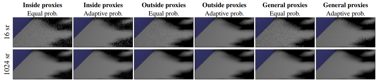
最小化开销
- \(\mathcal{P},\mathcal{P}'\) 都
hit 的时候,最小化方差会将 \(p_2\)
设置的很大
- 合理结果,因为此时第 2 项贡献最高,就是 \(V_{\mathcal{P}}(x,y)\)【看上面展开的式子即可】
- 但是其实我们希望多和 proxy 求交【更快】
- 我们求不出最好结果,给一个启发式
- \(f_1+f_4\) 表示二者一致程度,一致程度越高,越希望用 proxy【越希望只使用 \(p_1\)】
\[ \begin{aligned} p_1' &= 1-p_2'-p_3'\\ p_2' &= p_2\cdot\sqrt[4]{1-\left(f_1+f_4\right)}\\ p_3' &= p_3\cdot\sqrt[4]{1-\left(f_1+f_4\right)} \end{aligned} \]
Splitting the visibility
- 简单替换效果不好
- 考虑如下场景:所有物体都是 outside proxy,此时求交 \(x\) 始终在 bounding box 内部,于是 \(V_{\mathcal{P}'}(x,y)=0\)
- 此时估计退化为
\[ V_{\mathcal{P}}(x,y) = 0 + V_{\mathcal{P}}(x,y)\overline{0} - 0\cdot\overline{V_{\mathcal{P}}(x,y)} \]
- 进行如下拆分:\(x\)
所在的物体【包含的原体集合记作 \(\mathcal{O}\) 】
- \(x\) 所在物体的阴影检测使用标准的,外部使用 proxy
\[ \widetilde{V}(x,y) = V_{\mathcal{O}}(x,y)\cdot \widetilde{V}_{\mathcal{P}\setminus\mathcal{O}}(x,y) \]
- 使用 object instancing,\(\mathcal{O}\) 就是一个 object instance
实验
- 大的半影区域,使用 stochastic 算法不好
- 加速结构对这个处理很好
- 全影区域,使用原始几何和 proxy 效率差不多
- 收敛速度差不多
- 结果证明论文算法 MSE
其实都不如准确阴影计算
- 随机性能够支持更多 shadow ray,但是带来了更严重的噪声
- 16 probes rays 估计不够准,因此结果可能也不太好