(论文)[I3D-2018] Combining Analytic Direct Illumination and Stochastic Shadows

Combining Analytic Direct Illumination and Stochastic Shadows

• 主页【有代码实现】
• 提出了 ratio estimator
  • 把 DI 拆分为 unshadowed illumination x illumination-weighted shadow
  • 二者可以使用不同的技术进行计算
• 此外单独对阴影降噪【只会让 shadow 变模糊】，这样能够保留 shading 细节
• LTC 等方法能够很快计算不带阴影的光照，如果加上我们的阴影效果更好【多边形面光源】
• 完整光照表示
  • 直接拆分为不带阴影积分 x 阴影积分，结果是不正确的

\[ S=\int_{\Omega}\mathrm{BRDF}\times\mathrm{Light}\times\mathrm{Visibility} \]

• 本文：ratio estimator
  • U：analytic or precomputed
  • W：stochastic + denoising

\[ S = \underbrace{ \int_{\Omega} \mathrm{BRDF}\times\mathrm{Light} }_{\text{unshadowed illumination }U} \times \underbrace{ \frac{ \int_{\Omega}\mathrm{BRDF}\times\mathrm{Light}\times\mathrm{Visibility} }{ \int_{\Omega}\mathrm{BRDF}\times\mathrm{Light} } }_{\text{illumination-weighted shadow }W} \]

• 拆分好处
  • 只有 W 需要随机采样计算 => 只有阴影部分可能带噪声
  • U 可以保留完整细节（sharp shading details），不需要降噪

相关工作

• Unshadowed Direct Illumination
  • 快速解析计算
  • 预计算
• Ratio estimators：\(Y\) 的估计转化为 \(X,Y\) 的估计
  • 渐进意义下是无偏的，但是实际情况下都是有偏的
  • 正相关的时候，可能可以降方差【都偶然增大，偶然变小，方差降低】【考虑极端情况 \(Y=cX\)】
  • 【见最后的详细分析】

\[ \mathbb{E}[Y] = \lim_{N\to\infty} \frac{1}{N} \sum_{n=1}^{N} y_n \]

\[ \mathbb{E}[Y] = \mathbb{E}[X] \lim_{N\to\infty} \frac{ \sum_{n=1}^{N} y_n }{ \sum_{n=1}^{N} x_n } \]

• Control Variates【本文对比的时候，不借助额外预计算或数据结果，因此简单令 \(c=1\)】

\[ S = \underbrace{ c\int_{\Omega} \mathrm{BRDF}\times\mathrm{Light} }_{\text{control variate (analytic)}} - \underbrace{ \int_{\Omega} \mathrm{BRDF}\times\mathrm{Light}\times(c-\mathrm{Visibility}) }_{\text{error (stochastic)}}. \]

Ratio Estimator

• 简单表示
  • R：cosine-weighted BSDF
  • L：incident lighting
  • V：visibility
• 认为 U 能够快速计算

\[ S = \int_{\Omega} R(\omega)L(\omega)V(\omega)\,\mathrm{d}\omega, \qquad U = \int_{\Omega} R(\omega)L(\omega)\,\mathrm{d}\omega \]

• 原始估计

\[ S_N^{\mathrm{sto}} = \frac{1}{N} \sum_{n=1}^{N} \frac{ R(\omega_n)L(\omega_n)V(\omega_n) }{ p(\omega_n) } \]

• CV 估计【\(c=1\)】

\[ S_N^{\mathrm{CV}} = U - \frac{1}{N} \sum_{n=1}^{N} \frac{ R(\omega_n)L(\omega_n)(1-V(\omega_n)) }{ p(\omega_n) } \]

• 本文 Ratio Estimator
  • \(S_N^{\mathrm{sto}}\)、\(U_N^{\mathrm{sto}}\) 使用相同随机数：这样他们相除的结果能够保证在 \([0,1]\) 之间
  • 可以使用 MIS【本文：BSDF、NEE 都有】

\[ S_N^{\mathrm{ratio}} = U \times \frac{ S_N^{\mathrm{sto}} }{ U_N^{\mathrm{sto}} } \]

\[ U_N^{\mathrm{sto}} = \frac{1}{N} \sum_{n=1}^{N} \frac{ R(\omega_n)L(\omega_n) }{ p(\omega_n) } \]

• Ratio Estimator 是有偏的、一致的
  • 实验证明，能够降低方差【但是目前没有理论证明】
• 简单结果
  • CV 在暗区引入了亮噪点
  • 原始随机采样在亮区有明显噪点
  • 所有方法在软阴影边界有噪点

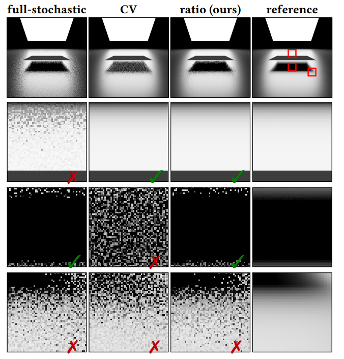
Approximate Ratio Estimators

• 节省带宽，计算 shadow 的时候使用 gray scale【不用 RGB】
  • 是一个近似，引入有偏性
• 不带阴影的直接光估计
  • 假设可以解析计算、或者预计算
  • 复杂 BSDF 很难【实时一般近似】

\[ \int_{\Omega}\tilde{R}L \neq \int_{\Omega}RL \]

• 但是我们在计算 weighted 项的时候使用原始材质 \(R\) 更方便，在这种近似下

\[ \int_{\Omega} \tilde{R}L \times \frac{ \int_{\Omega}RLV }{ \int_{\Omega}RL } \neq \int_{\Omega}RLV \]

• 在实时场景下，这样的近似效果还行

Denoising the Ratio Estimator

• 先对 \(S_N^{\mathrm{ratio}}\)、\(U_N^{\mathrm{ratio}}\) 进行降噪，再把他们相除

\[ \frac{ \mathrm{denoise}[S_N] }{ \mathrm{denoise}[U_N] } \longrightarrow \frac{S}{U} \]

• 对结果降噪

\[ \mathrm{denoise} \left[ \frac{S_N}{U_N} \right] \nrightarrow \frac{S}{U} \]

• 这部分解释感觉有点怪，感觉如果降噪器都是随着 \(N\to\infty\) 没有误差的话，应该都是一致的
• 先降噪的话，出现 0/0=NaN 情况少【因为和邻居像素 mix 了】
  • 不能直接特殊处理吗？
• 降噪：简单双边滤波
  • 不用 SVGF，在差的降噪器上，更能显示鲁棒性【开始胡扯了】
• 降噪的好处【和全随机相比】
  • sharp shading + blurred shadow【因为只对 shadow 降噪了】
  • 【CV】因为暗区有亮噪点，直接把阴影部分搞没了

实时算法

算法流程

• 计算带噪结果，下一步高斯核标准差正比于 \(E\)【大小和标准差相关】【具体在下面】
  • Compute the noise estimate \(E\) from \(W_N=\dfrac{S_N}{U_N}\)
  • Denoise \(E\) itself via a \(3\times3\) box filter
• 分别降噪出结果【2 pass】：Gaussian kernel with the bilateral weights
  • Horizontally joint-bilateral filter \(S_N\) and \(U_N\) simultaneously【同时计算，减小读 G-Buffer 开销】
  • Vertically joint-bilateral filter \(S_N\) and \(U_N\) simultaneously and produce a single output: final image \(U\times\dfrac{\mathrm{denoise}[S_N]}{\mathrm{denoise}[U_N]}\)
• 时域降噪【SIG15 的 course】
  • Temporally integrate the final image via reverse reprojection

噪声估计

• 估计 \(E\)
• 只是计算方差是不准确的，没有考虑顺序
  • 例如冲激函数（可能是阴影边界的噪声）、阶跃函数（需要保留的硬阴影边界）
• 本文：评估 \(W_N\) 的颜色梯度变化快慢
  • \(S_N\approx0,U_N\approx0\) 的时候，设置 \(W_N=1\)
  • 使用 4 条直线【0/45/90/135 度，两端延伸；然后每个像素使用随机角度偏移】
    • 引入噪声，box filter

\[ E[x] = \frac{1}{n} \sum_{i} \int_{\ell_i} \left\| \frac{ \mathrm{d}^2 W_N[\ell_i(t)] }{ \mathrm{d}t^2 } \right\| \,\mathrm{d}t \]

• \(E[x]\) 只有在噪声比较重的区域，值比较高【软阴影区域】
  • 硬阴影边界小一些【只有一个方向上的少量像素梯度变化大】
• \(E\) 只对应半影区域

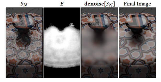
Real-Time Area Lights

• LTC 计算 \(U\)
• deferred shading pass ：渲染 G-Buffer
  • \(N\) spp：3 张 \(N\) 倍大小的 texture
    • shadow ray origins + start distance offset
    • shadow ray directions + end distance
    • radiance
  • 此时 \(U,U_N\) 已经能够计算了
• 计算 \(S_N\)：投射所有 shadow ray，然后累计没被遮挡的贡献
• MIS：NEE + BRDF rays
• 蓝噪声

Ratio Estimator 详细分析

• Ratio Estimator（比率估计量）

\[ \widehat{\mu}_Y^{\mathrm{ratio}} = \mu_X\frac{\overline{Y}}{\overline{X}} = \mathbb{E}[X] \frac{\sum_{n=1}^{N}y_n}{\sum_{n=1}^{N}x_n} \]

• 其中

\[ \overline{Y} = \frac{1}{N}\sum_{n=1}^{N}y_n, \qquad \overline{X} = \frac{1}{N}\sum_{n=1}^{N}x_n \]

• 并且 \(\mu_X=\mathbb{E}[X]\) 已知

渐近无偏

• 在满足大数定律且 \(\mathbb{E}[X]\neq 0\) 的情况下，

\[ \overline{X}\to\mu_X, \qquad \overline{Y}\to\mu_Y \]

• 因此在渐近意义下是正确的【一致估计量】

\[ \mu_X\frac{\overline{Y}}{\overline{X}} \to \mu_X\frac{\mu_Y}{\mu_X} = \mu_Y \]

• 更严谨地应写成

\[ \widehat{\mu}_Y^{\mathrm{ratio}} = \mu_X\frac{\overline{Y}}{\overline{X}} \xrightarrow[N\to\infty]{} \mu_Y \]

降低方差

• 仅仅满足正相关【\(\operatorname{Cov}(X,Y)>0\)】，并不能保证 Ratio Estimator 的方差一定小于普通样本均值

• 一阶 Taylor 展开

\[ \mu_X\frac{\overline{Y}}{\overline{X}} \approx \overline{Y} - \frac{\mu_Y}{\mu_X} \left( \overline{X}-\mu_X \right) \]

• 因此，其渐近方差约为

\[ \operatorname{Var} \left[ \widehat{\mu}_Y^{\mathrm{ratio}} \right] \approx \frac{1}{N} \operatorname{Var} \left( Y-\frac{\mu_Y}{\mu_X}X \right) \]

\[ \operatorname{Var} \left[ \widehat{\mu}_Y^{\mathrm{ratio}} \right] \approx \frac{1}{N} \left[ \operatorname{Var}(Y) + \left( \frac{\mu_Y}{\mu_X} \right)^2 \operatorname{Var}(X) - 2\frac{\mu_Y}{\mu_X} \operatorname{Cov}(X,Y) \right] \]

• 而普通估计量的方差为

\[ \operatorname{Var}[\overline{Y}] = \frac{\operatorname{Var}(Y)}{N} \]

• 所以 Ratio Estimator 降低方差需要满足

\[ \left( \frac{\mu_Y}{\mu_X} \right)^2 \operatorname{Var}(X) - 2\frac{\mu_Y}{\mu_X} \operatorname{Cov}(X,Y) <0 \]

• 如果

\[ \frac{\mu_Y}{\mu_X}>0 \]

• 则可以写成

\[ \frac{\mu_Y}{\mu_X} < 2\frac{\operatorname{Cov}(X,Y)} {\operatorname{Var}(X)} \]

• 因此，正相关是有利条件，但不是充分条件

• 更准确的说法是：当 \(Y\) 与 \(X\) 近似成比例，并且两者具有较强正相关性时，Ratio Estimator 通常可以降低方差

通常是有偏的

• Ratio Estimator 在有限样本下通常不是无偏估计量：

\[ \mathbb{E} \left[ \mu_X\frac{\overline{Y}}{\overline{X}} \right] \neq \mu_Y \]

• 原因是一般有

\[ \mathbb{E} \left[ \frac{\overline{Y}}{\overline{X}} \right] \neq \frac{\mathbb{E}[\overline{Y}]} {\mathbb{E}[\overline{X}]} \]

• 通过二阶 Taylor 展开，其偏差近似为

\[ \operatorname{Bias} \left[ \widehat{\mu}_Y^{\mathrm{ratio}} \right] \approx \frac{1}{N} \left[ \frac{\mu_Y}{\mu_X^2}\operatorname{Var}(X) - \frac{1}{\mu_X}\operatorname{Cov}(X,Y) \right] \]

• 这个偏差通常是 \(O\left(\dfrac{1}{N}\right)\)，所以随着样本数增大趋于零

与 Control Variate 的关系

• 一阶展开为

\[ \widehat{\mu}_Y^{\mathrm{ratio}} \approx \overline{Y} - \frac{\mu_Y}{\mu_X} \left( \overline{X}-\mu_X \right) \]

• 这正是一个 Control Variate 形式

\[ \widehat{\mu}_Y^{\mathrm{CV}} =\overline{Y}-\beta\left(\overline{X}-\mu_X\right) =\beta\mu_{X}-\left(\overline{Y}-\beta\overline{X}\right) \]

• 其中，Ratio Estimator 隐式使用

\[ \beta_{\mathrm{ratio}} = \frac{\mu_Y}{\mu_X} \]

• 而 Control Variate 的最优系数是【写出方差，然后对 \(\beta\) 求导】

\[ \beta^* = \frac{\operatorname{Cov}(X,Y)} {\operatorname{Var}(X)} \]

• 所以 Ratio Estimator 效果好的本质条件是

\[ \frac{\mu_Y}{\mu_X} \approx \frac{\operatorname{Cov}(X,Y)} {\operatorname{Var}(X)} \]

• 这通常对应于 \(Y\) 和 \(X\) 近似满足过原点的线性关系

\[ Y\approx cX \]

其他

泰勒展开

• 一阶泰勒展开

\[ g(x,y) \approx g(x_0,y_0) + \frac{\partial g}{\partial x}(x_0,y_0)(x-x_0) + \frac{\partial g}{\partial y}(x_0,y_0)(y-y_0) \]

• \(g(x,y)=a\dfrac{y}{x}\) 的一阶泰勒展开为

\[ g(x,y) \approx g(x_0,y_0) - a\frac{y_0}{x_0^2}(x-x_0) + \frac{a}{x_0}(y-y_0) \]

• 多阶泰勒展开【其中 \(R_m\) 是余项】

\[ g(x,y) = \sum_{\substack{i,j\ge 0,i+j\le m}} \frac{1}{i!j!} \frac{\partial^{i+j}g}{\partial x^i\partial y^j}(x_0,y_0) (\Delta x)^i(\Delta y)^j + R_m \]

方差展开

• 代入原始定义展开即可

\[ \operatorname{Var}[X+Y] = \operatorname{Var}[X] + \operatorname{Var}[Y] + 2\operatorname{Cov}(X,Y) \]

\[ \operatorname{Cov}(X,Y) = \mathbb{E}\left[ \left(X-\mathbb{E}[X]\right) \left(Y-\mathbb{E}[Y]\right) \right] \]