(论文)[2025-SIG] Segment-based Light Transport Simulation
Segment-based Light Transport Simulation
Wenyou Wang、Rex West、Toshiya Hachisuka
- 1、3:University of Waterloo, Canada
- 2:Aoyama Gakuin University, Japan
代码:好像只有空仓
贡献
新渲染框架:以 segment 作为基本元素,而不是 vertex
采样框架基于 MMIS
验证:实现了 robust bidirectional path filtering method
Background
- 渲染方程
- \(\bar{\mathrm{x}} = \{ \mathrm{x}_1, \ldots, \mathrm{x}_k \}\)
 \[
I_{\rho} = \int_{\mathcal{P}} f_{\rho}(\mathrm{\bar{x}})
\,\mathrm{d}\mathrm{\bar{x}} = \sum_{k=1}^{\infty}
\underbrace{\int_{\mathcal{P}_k} f_{\rho}(\mathrm{\bar{x}})
\,\mathrm{d}\mathrm{\bar{x}}}_{= I_k} \tag{1}
\]
\[
I_{\rho} = \int_{\mathcal{P}} f_{\rho}(\mathrm{\bar{x}})
\,\mathrm{d}\mathrm{\bar{x}} = \sum_{k=1}^{\infty}
\underbrace{\int_{\mathcal{P}_k} f_{\rho}(\mathrm{\bar{x}})
\,\mathrm{d}\mathrm{\bar{x}}}_{= I_k} \tag{1}
\]
\[ f_{\rho}(\bar{\mathrm{x}}) = W_{\rho}(\mathrm{x}_1, \mathrm{x}_2) \prod_{i=1}^{k} G(\mathrm{x}_i, \mathrm{x}_{i+1}) \prod_{i=2}^{k-1} f_r(\mathrm{x}_{i-1}, \mathrm{x}_i, \mathrm{x}_{i+1}) L_e(\mathrm{x}_{k-1}, \mathrm{x}_k) \tag{2} \]
Disconnected Subpaths
- BDPT
- PM:收集周围光子 \(\mathrm{x}_2\) 收集 \(\mathrm{x}_2'\),构建新光路
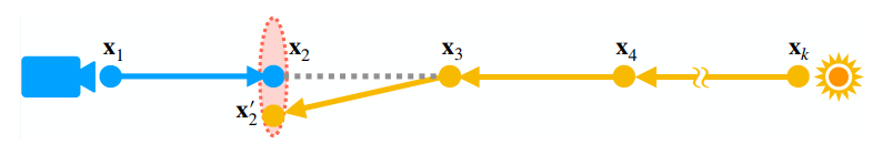
- Path filtering
- UPT 框架中,收集 kernel 内的前缀路径,连接他们的后缀路径形成新路径
- SMIS 将 path filtering 看成一个采样过程:前缀是 technique,新路径是 sample
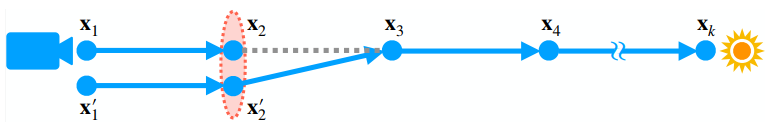
Paths to Segments
- 之前的做法都是让其归约到传统 PT,采样后移除多余节点
- VCM:kernel 内部采样【rejection sampling process】
- SMIS:对前缀路径(technique)采样
- UPS:连接 disconnected subpaths
- 以 segment(节点对)为单位,light transport(根据连接概率)
- 后续发展少(segment sampling,segment path construction)
Segment-Based Light Transport
- 基于线段【segment】积分的框架【第一个】
Formulation
- 积分形式
\[ J_{\rho} = \int_{\mathcal{S}} g_{\rho}(\bar{\text{s}}) \, \mathrm{d}\bar{\text{s}} = \sum_{k=1}^{\infty} \underbrace{\int_{\mathcal{S}_k} g_{\rho}(\bar{\text{s}}) \, \mathrm{d}\bar{\text{s}}}_{= J_{\rho,k}} \]
- \(\rho\):像素
- \(\mathcal{S}_k=\mathcal{M}^{2k}\):长度为
\(k\) 的线段 \(\bar{\text{s}} = \{ \text{s}_1 \ldots \text{s}_k
\}\) 的集合
- \(\text{s}_i=(\mathrm{x}_i,\mathrm{y}_i)\)
- \(g_{\rho}(\bar{\text{s}})\) 是对像素的贡献
\[ g_{\rho}(\bar{\text{s}}) = W_{\rho}(\text{s}_1) \prod_{i=1}^{k} G(\text{s}_i) \prod_{i=1}^{k-1} K(\text{s}_i, \text{s}_{i+1}) f_r(\text{s}_i, \text{s}_{i+1}) L_e(\text{s}_k) \]
- 相机敏感度函数 \(W_{\rho}(s) = W_{\rho}(x_1, y_1)\)
- kernel 函数 \(K(\text{s}_i, \text{s}_{i+1})\)
- 几何项 \(G(\text{s}_i)\)
\[ G(\text{s}_i)=\frac{|\mathrm{n}_{\text{x}_i} \cdot \bar{\text{s}}_i| \, |\mathrm{n}_{\text{y}_i} \cdot \bar{\text{s}}_i|}{|\text{x}_i - \text{y}_i|^2} V(\text{x}_i, \text{y}_i) \]
- 自发光项 \(L_e(\text{s}_k) = L_e(\text{x}_k, \text{y}_k)\)
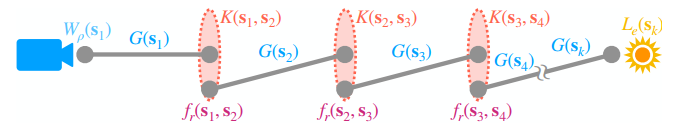
- 注意
- \(W,G,L\) 只和线段本身相关【不变的】
- \(K,f_{r}\) 和相邻的线段相关
kernel 函数
- \(K\)
的设计允许和方向相关,而不是简单的两个顶点
- 可以任意给定,只需要满足能量守恒
\[ \int_{\mathcal{M}} K(\text{s}_i, \text{s}_{i+1}) \, \mathrm{d}\text{x}_{i+1} = 1 \tag{5} \]
- 本文:有限范围内的均匀分布
- 类似 PM,如何选择 Kernel 可以是后续工作
\[ K(\text{s}_i, \text{s}_{i+1}) = \left( \int_{\mathcal{K}(y_i)} \mathrm{d}\text{x}_{i+1} \right)^{-1} \]
- 当 \(K\) 是 Delta 分布的时候,我们的算法退化到之前的基于顶点的表达
Throughput function
- 为了和 Delta 时保持一致,当 \(\mathrm{x}_i=\mathrm{y}_{i+1}\) 的时候,退化为三元组
\[ f_r(\text{s}_i, \text{s}_{i+1})=f_r(\text{x}_i, \text{y}_i, \text{y}_{i+1}) \]
- 我们提出 shift invariant【不变量】
- \(\text{x}_{i+1}\) 依赖于 \(\text{y}_{i}\)
- 和 path filtering 一致:不做方向修正的复用 incident radiance
\[ f_r(\text{s}_i, \text{s}_{i+1})=f_r(\text{x}_i, \text{y}_i, \text{y}_{i+1}-(\text{x}_{i+1},\text{y}_{i})) \]
- 论文使用 shift invariant,其他作为后续工作
- 将渲染方程展开为递归形式
\[ L(\text{s}) = L_e(\text{s}) + \int_{\mathcal{S}_1} K(\text{s}, \text{s}') f_r(\text{s}, \text{s}') G(\text{s}') L(\text{s}') \, \mathrm{d}\text{s}' \tag{7} \]
\[ J_\rho = \int_{\mathcal{S}_1} W_\rho(\text{s}) G(\text{s}) L(\text{s}) \, \mathrm{d}\text{s} \tag{8} \]
Segment Samplers and Estimators
Samplers
- 采样示意图
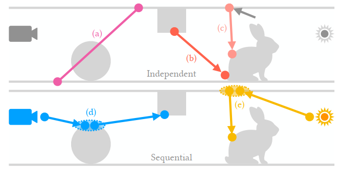
Uniform segment sampler
- 上图的 (a)
- 随机采样两个点,然后连起来
- \(|\mathcal{M}|\) 表示场景面积
\[ p(\text{s}) = p(\text{x}) p(\text{y}) = \frac{1}{|\mathcal{M}|^2} \tag{12} \]
- impractical,无重要性采样,低效
Ray tracing segment sampler
- 稍改进一些
- 第一个随机采,第二个点 cosine 半球采样
- 需要从立体角转化度量为面积度量
\[ p(\text{s}) = p(\text{x}) p(\text{y} \mid \text{x}) = \frac{1}{|\mathcal{M}|} \cdot \frac{|\mathrm{n}_{\text{x}_i} \cdot \vec{\text{s}}_i| \, |\mathrm{n}_{\text{y}_i} \cdot \vec{\text{s}}_i|}{\pi |\text{x} - \text{y}|^2} = \frac{G(\text{s})}{\pi |\mathcal{M}|} \tag{13} \]
- 结果上来说重要性采样了几何项 \(G(\text{s})\)
- 上图的 (b)
- 直接重要性采样 \(\mathrm{x}\)
的BSDF:上图的 (c)
- \(p(\bar{\text{s}} \mid \text{x}, \bar{\text{s}}')\) 正比于 BSDF,立体角度量分布
\[ p(\text{s} \mid \bar{\text{s}}') = p(\text{x}) p(\text{y} \mid \text{x}, \bar{\text{s}}') = \frac{1}{|\mathcal{M}|} \cdot \frac{p(\bar{\text{s}} \mid \text{x}, \bar{\text{s}}') \, |\mathrm{n}_{\text{y}_i} \cdot \bar{\text{s}}|}{|\text{x} - \text{y}|^2} \tag{14} \]
- 上面方法的问题:segment 独立采样【效率低】
Sequential segment sampler
- 类似于【path tracing、light tracing】
- 采样一个序列【上图的 (d) (e)】
- 初始
- path tracing:\(p_W(\text{s}_1) \sim W_{\rho}(\text{s}_1) G(\text{s}_1)\)
- light tracing:\(p_L(\text{s}_1) \sim L_e(\text{s}_1) G(\text{s}_1)\)
- 后续 segment
- 按照 kernel 采样第一个点:\(p_K(\text{x}_{i+1}\mid\text{s}_i)\sim K(\text{s}_i,\text{s}_{i+1})\)
- 按照 BSDF 采样第二个点
$$
- virtual perturbation:复制 \(\mathrm{x}_{i+1}=\mathrm{y}_{i}\)
- 保留 pdf \(p_K(\text{x}_{i+1}\mid\text{s}_i)\)【这样估计之后就不是无偏的了吧】
- bridge segment:采样的线段【区别于传统的确定性连接】
- 只是这样,没有带来好处
Estimators
- 和 vertex 不同,segment 的采样方式不需要知道【给了更大的自由度】
- 给一些基础算法
Sequential
- 采样 \(k\) 个线段
\[ \langle J_{\rho k} \rangle = \frac{g_{\rho}(\bar{\text{s}})}{p(\bar{\text{s}})},\quad p(\bar{\text{s}}) = p(\text{s}_1, \ldots, \text{s}_k) \tag{16} \]
Multiple sampling techniques
- BDPT 启发
- \(T\) 种采样技术,每种采样技术 \(n_i\) 个样本
\[ \langle J_{\rho k} \rangle_{\text{MIS}} = \sum_{i=1}^{T} \sum_{j=1}^{n_i} \frac{w_i(\bar{\text{s}}_{i,j}) g_{\rho}(\bar{\text{s}}_{i,j})}{n_i p_i(\bar{\text{s}}_{i,j})} \tag{17} \]
- 只需要满足对于所有路径:\(\sum_{i=1}^{T}w_i(\bar{\text{s}})=1\) 即可
Recursive estimation
\[ \langle L(\text{s}) \rangle_{\text{BH}} = L_e(\text{s}) + \sum_{i=1}^{T} \sum_{j=1}^{n_i} \frac{K(\text{s}, \text{s}_{i,j}') f_r(\text{s}, \text{s}_{i,j}') G(\text{s}_{i,j}') \langle L(\text{s}_{i,j}') \rangle_{\text{BH}}}{\sum_{i'=1}^{T} \sum_{j'=1}^{n_{i'}} p_{i'}(\text{s}_{i,j}' \mid t_{i',j'})} \tag{18} \]
- pixel forming equation【式子 8】
\[ \langle J_{\rho} \rangle_{\text{BH}} = \sum_{i=1}^{T} \sum_{j=1}^{n_i} \frac{W_{\rho}(\text{s}_{i,j}) G(\text{s}_{i,j}) \langle L(\text{s}_{i,j}) \rangle_{\text{BH}}}{\sum_{i'=1}^{T} \sum_{j'=1}^{n_{i'}} p_{i'}(\text{s}_{i,j} \mid t_{i',j'})} \tag{19} \]
- 直接展开有植树问题:使用 multi-vertex path filtering 高效实现
- 类似 Path Graph / MMIS
Marginal segment path sampling
- 不是所有的都适合递归展开
- MMIS 对于整条路径的版本
\[ \langle J_{\rho k} \rangle_{\text{BH}} = \sum_{i=1}^{\bar{T}} \sum_{j=1}^{n_i} \frac{g_{\rho}(\bar{\text{s}}_{i,j})}{\sum_{i'=1}^{\bar{T}} \sum_{j'=1}^{n_{i'}} p_{i'}(\bar{\text{s}}_{i,j} \mid \bar{t}_{i',j'})} \tag{20} \]
Practical Algorithm
Segment-based path tracing
- sequential segment sampler + sequential estimation
- 避免单向的问题:BSDT + bridge segment【MIS】
- 效果比不过 vertex-based,没有发挥 segment 的优势
Segment-based multi-vertex path filtering
- path filtering 的 segment 版本
- 参考 MMIS 的 path filtering
- 相机出发:multi-vertex filtering(MVF)
- 光源出发:photon filtering(PhF)
Bidirectional path filtering
- 基于 vertex 的版本很难实现 bidirectional filtering【不确定?】
- 基于线段的算法能够天然的处理来自于任意分布
- 直接两头出发 sequential sampling,然后使用 MMIS 连接

- 是 bidirectional photon mapping 的超集
- kernel 的帮助下非常鲁棒
实验与讨论
- CPU-based RGB renderer
- 设定
- 1200 x 800
- segment path depth = 8
- 1 segment path per pixel【per iteration】
- light paths / camera paths:\(\beta=0.25\)
- kernel 初始大小:4x average pixel footprint
- \(\alpha=0.67\) 缩圈
Bidirectional Filtering
- 同时间对比:MVF、PhF、BPM、UPS
- 说是 MVF 一致的比 PT 好,所以不加 PT
- 类似的原因不比 BDPT【但是感觉 UPS 不一定比 BDPT 好吧,而且 BDPT 后续发展还很多】
- 复杂场景:\(\beta=1.0\)
- 结果上来说
- MVF、PhF【单向】存在优势场景,但是有明显的失败场景
- BPM、UPS【双向】收敛没有我们快
其他实验
- Filtering Efficiency and Kernel Size
- 大 kernel 收敛快,bias 大;小 kernel 收敛慢
- PPM 类似的缩半径策略做到了平衡
- Path Reuse Efficiency
- 和 BPM 相比,我们是超集;不同的 \(\beta\)
- 我们一致的好
- \(\beta\) 增大,MMIS 的平方计算开销导致很大的 \(\beta\) 结果反而不一定好
- Adding Bridge Segments【具体看补充材料】
- 同时间差;同样本好【平方计算代价高】
- 【留给 future work】
未来工作
- Segment sampling
- path guiding
- MCMC
- 和 vertex-based sampler 结合
- bridge segment 的重要性采样
- 类似 BDPT 的概率链接
- Segment paths construction
- 泛化成 directionaless variant
- Path filtering
- MMIS 平方计算量
- 如何提高 filtering efficiency
- Temporal Filtering
补充材料
Bridge Segment Sampler
- 最简单的策略:kernel 采样两个点,然后可见性测试连起来
\[ p(\text{s}_i \mid \text{s}_{i-1}, \text{s}_{i+1}) = p(\text{s} \mid \text{z}_{i-1}, \text{z}_{i+1}) = p_K(\text{x}_i \mid \text{z}_{i-1}) p_K(\text{y}_i \mid \text{z}_{i+1}) \tag{S6} \]
- 类似 NEE,可以对光源(相机)采样
- kernel 采样一个点;然后光源(相机)采样一个点
\[ p(\text{s}_i \mid \text{s}_{i-1}) = p(\text{s} \mid \text{z}_{i-1}) = p_W(\text{x}_i) p_K(\text{y}_i \mid \text{z}_{i-1}) \tag{S7} \]
\[ p(\text{s}_i \mid \text{s}_{i-1}) = p(\text{s} \mid \text{z}_{i-1}) = p_L(\text{x}_i) p_K(\text{y}_i \mid \text{z}_{i-1}) \tag{S8} \]
MMIS
- 采样 techinque、sample 对 \((t_i,s_i)\),然后做 MIS
- 具体看 MMIS
实现细节
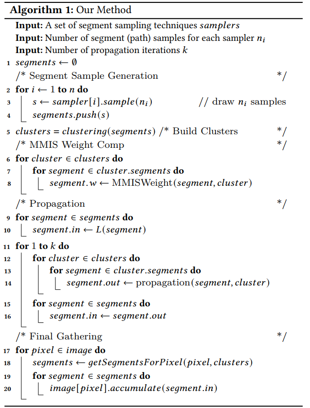
- 核心:segment samplers、clustering algorithms、propagation
- 每轮迭代
- 采样线段
- 线段顶点聚类
- 传播线段 throughput
- 采样线段:sequential segment samplers + bridge segment sampler
- virtual perturbation【拷贝顶点】
- 就是和传统的差不多
- 聚类
- kernel:uniform kernel
- 定义域由 position-normal voxel encoding method 决定【spatial hashing 常用,不懂】
- 保存所有线段端点的哈希值
- 根据哈希值排序,实现聚类
- 类内顶点使用相同定义域
- 量化误差使用 jittering 转化为噪声
- 评估 kernel 函数:计算 voxel 内部的平均位置、法向
- 值设置为位置、法向张成平面和 voxel 的相交面积的倒数【也不太懂】
- 这样估计会有扁案的 bias;缩 voxel 能解决
- kernel:uniform kernel
- 传播
- 预先计算 MMIS 权重,每一个线段最多和两个类别相关
- 与计算完之后迭代计算,传播
- 大概懂思路,具体细节还得看他开源代码