(论文)[2024-SIG-C] Neural Product Importance Sampling via Warp Composition

Neural Product Importance Sampling via Warp Composition

• 主页
• 作者：Joey Litalien, Miloš Hašan、Fujun Luan、Krishna Mullia、Iliyan Georgiev
  • McGill University，Adobe Research

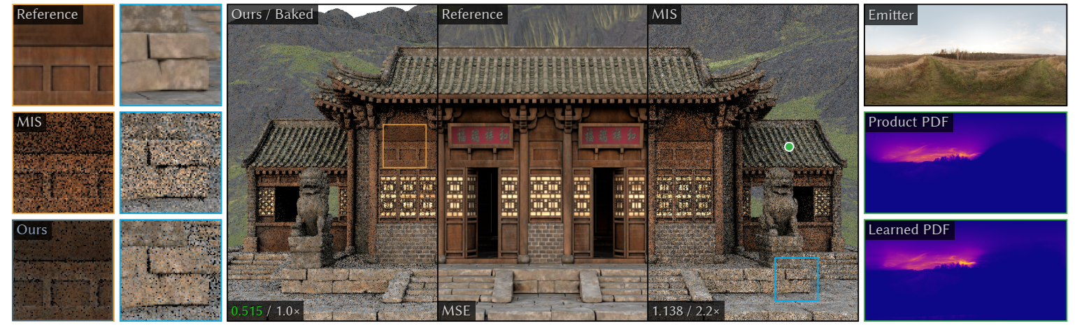
• 摘要：如何结合材质采样、光源采样；我们的方法比 MIS 更好
  • small conditional head warp：neural spline flow
    • 低维也能离散化
  • large unconditional tail warp：discretized【离散】

• 环境光源 DI 的 path guiding：期望最终的采样分布近似于分子【单材质训练】
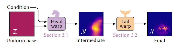
  • 分布通过两步变换完成【head warp + tail warp】
    • 都是通过 normalizing flow 实现
    • head 是小的条件 NF，tail 是大的无条件 NF
  • 先训练 tail warp 将 unifrom 分布转化为环境光分布
  • 然后固定 tail warp，针对场景的每个材质进行训练 head warp，使得最终的分布和分子相近
    • 不考虑阴影
    • 【我感觉应该是每个物体每个材质】不过环境光似乎不需要单物体，只和 view direction 有关了
• 为了加速，tail warp 的变换/逆变换离散化

Background and Related Work

• Monte Carlo integration
  • \(\perp\)：cosine-weighted BSDF

\[ L_o(\mathbf{x}, \omega_o) = \int_{\Omega} f_r^{\perp}(\mathbf{x}, \omega_o, \omega) \, L(\omega) \, V(\mathbf{x}, \omega) \,\mathrm{d}\omega \tag{1} \]

\[ \langle L_o \rangle_N = \frac{1}{N} \sum_{i=1}^{N} \frac{f_r^{\perp}(\mathbf{x}, \omega_o, \omega_i) \, L(\omega_i) \, V(\mathbf{x}, \omega_i)}{p(\omega_i \vert \mathbf{x}, \omega_o)}, \omega_i \sim p \tag{2} \]

• MIS 比估计乘积效果差，而且可能会过于保守
• Product importance sampling
  • 我们方法样本少的时候，效果也好
• Resampled importance sampling
  • RIS 可以叠在我们方法上，进一步提高效果
• 变换分布
  • 【EGSR-2020】Practical Product Sampling by Fitting and Composing Warps
  • 和我们很像，但是他们求解的是面光源、解析变换
• Normalizing flows【NFs】
  • 分布变换：简单的基本分布 \(p_{\mathcal{Z}}\)；复杂的目标分布 \(p_{\mathcal{X}}\)
  • 变换使用网络拟合，可微可逆双射 \(f:\mathcal{Z}\to\mathcal{X}\)
    • \(\theta\) 表示 \(f\) 的参数

\[ p_{\mathcal{X}}(x; \theta) = p_{\mathcal{Z}}(z) \, \lvert J_f(z; \theta) \rvert^{-1} \tag{3} \]

\[ J_f(z;\theta) \triangleq \det\left( \frac{\partial f(z; \theta)}{\partial z^T} \right) ,z \sim p_{\mathcal{Z}} \]

\[ z=f^{-1}(x;\theta) \]

• 优化 \(\theta\) 一般使用分布差异度量（例如 KL 散度）
  • 训练的时候能获取 \(x\sim p_{\mathcal{X}}^{\ast}\) 的话，等价于最大似然估计
• neural spline flows：换了一种变换形式【更鲁棒】
• Neural sampling for rendering
• 环境光源的获取只需要一个方向

Neural Warp Composition

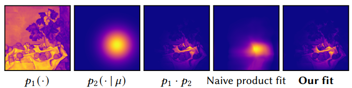
• 目的：\(p^{*}(x \vert c) \propto p_1(x) \cdot p_2(x \vert c)\)
• 假定
  • \(p_1\) 复杂（例如 an unshadowed environment map ）
  • \(p_2\) 简单（例如 BSDF）
• 不去近似可见性【这是 scene-specific】
• 实时性能要求模型较小，这导致直接近似效果差
  • image intensity x Gaussian 例子

• 拆分，使用变换
  • \(h,t\) 及其逆都是连续的

\[ f(z \vert c; \theta) \triangleq (t \circ h)(z \vert c; \theta) = t(h(z \vert c; \theta)) \tag{4} \]

• 记号
  • target 分布：\(p^{\ast}\)
  • 学习的分布：\(p\)
• Application to rendering
  • \(p_1\)：unshadowed environment light
  • \(p_2\)：cosine-weighted BRDF
  • \(c\triangleq(\omega_o,n,\rho)\)
  • \(\mathcal{X}=\mathcal{Y}=\mathcal{Z}=[0,1]^2\)
  • 最后 lat-long warp 转化为 \(\omega\)

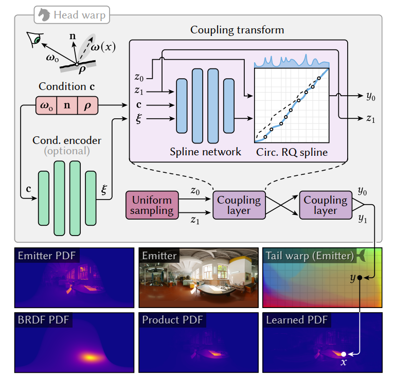
Neural-flow head warp

• 使用 neural spline flows 构建 \(h\)，使用其
  • utilize monotonic piecewise rational-quadratic splines as quantile functions（inverse CDFs） to warp samples
  • 单调分段有理二次样条
• 和标准的 NF 不同，\(p_{\mathcal{Z}}=\mathcal{U}[0,1]^2\)【标准 NF 不支持】
• 流程如下，两个 coupling layer 结构相同【只是结构相同，是参数独立的两个网络】
  • 网络 1 输入为 \((c,\xi,z_0,z_1)\)，网络 2 输入为 \((c,\xi,z_1,y_0)\)
  • 输入为 \(y=h(z)\)，喂给 Tail Warp

• 和 NeuSample 的区别
  • 架构不同
  • 参数化
    • global（cylindrical）equi-rectangular parameterization
    • NeuSample：local shading-point hemisphere（projected onto a square）
  • 我们保证 \(y,z\) 双射，但是 NeuSample 学一个圆盘边界丢弃越界样本

Tail warp

• \(y\) 先映射到 unit-square points \(x\in\mathcal{X}\)【根据 HDR 环境光】，然后 lat-long 投影到球面
  • 传统的方式虽然快，但是是离散的，不利于优化
    • marginal row column scheme
    • hierarchical
• 对环境光使用大的 NF 进行近似
  • spline-based flow【保证平滑】
  • 可以使用上面两种任意一种进行训练，增加 bins 可以减小误差
  • 考虑过 optimal-transport（OT）map ，但是效果不好【regularization 计算需要 env 平滑，但是这不实际】
• 我们训完 tail NF 之后，将其离散化（包括 forward and inverse warps）（at high resolution）
  • 这样采样和 pdf evaluation 就变成了查表+线性插值【快】
  • 这也离散化，为啥比之前离散化好
• tail warp 的作用：transform uniform density to the emitter-image density
• 训练
  • 先训练 tail warp，将均匀分布转化为环境光分布
  • 再训练 head warp，优化其使得 tail warp 的输出满足 product 分布【此时 tail 不变】

Head-warp training

• 使用 KL 散度训练
  • \(p(z)\) 是 uniform 分布
  • 省略了条件 \(c\)

\[ \begin{align} \mathcal{L}_{\text{KL}}(\theta) &= D_{\text{KL}} \left[ p_{\mathcal{X}}^{*}(x) \,\big\|\, p_{\mathcal{X}}(x; \theta) \right] \tag{5} \\ &= -\mathbb{E}_{x \sim p_{\mathcal{X}}^{*}} \left[ \log p_{\mathcal{X}}(x; \theta) \right] + \text{const} \tag{6} \\ &= -\mathbb{E}_{x \sim p_{\mathcal{X}}^{*}} \left[ \log \lvert J_f(z; \theta) \rvert^{-1} \right] + \text{const} \tag{7} \end{align} \]

• \(f=t\circ h\)，逆变换 \(f^{-1}=h^{-1}\circ t^{-1}\)

\[ \begin{align} \log \lvert J_f(z; \theta) \rvert^{-1} &= \log \lvert J_t(h(z; \theta)) J_h(z; \theta) \rvert^{-1} \tag{8} \\ &= \log \lvert J_t(h(z; \theta)) \rvert^{-1} + \log \lvert J_h(z; \theta) \rvert^{-1} \tag{9} \\ &= \log \lvert J_{t^{-1}}(x) \rvert + \log \lvert J_{h^{-1}}(t^{-1}(x); \theta) \rvert \tag{10} \end{align} \]

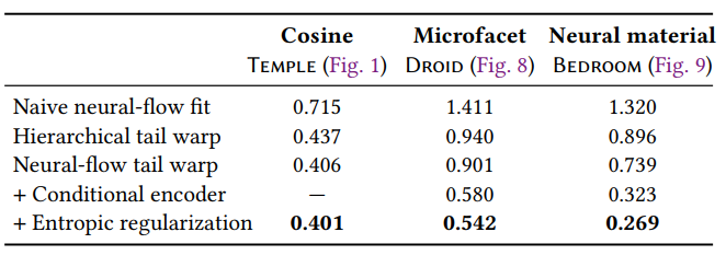
Entropic regularization

• KL 散度容易让分布在 high density 部分过度拟合，导致 low density 部分拟合效果差
  • MC 噪声大，对 fireflies 敏感
• \(\chi^2\) 更好，对 fireflies 不太敏感；但是过于保守
• 我们为 KL 加上正则项【这里 arxiv 上修正了，acm 上甚至写错了，离谱】
  • \(p\) 特别大的时候，加上一个反向梯度
  • \(\lambda=0.0001\)

\[ \begin{align} \mathcal{L}(\theta) &= \mathcal{L}_{\text{KL}}(\theta) + \lambda \mathcal{L}_{\text{H}}(\theta)\tag{11} \\ \\ \text{where }\mathcal{L}_{\text{H}}(\theta) &= \mathbb{E}_{x \sim p_{\mathcal{X}}^*} \left[ p_{\mathcal{X}}(x; \theta) \log p_{\mathcal{X}}(x; \theta) \right] \tag{12} \end{align} \]

讨论

• 我们的训练，需要样本满足 \(x\) 满足于目标分布 \(p^{\ast}\)【咋实现？下面有说，离散打表求解】
• 可以用 reverse KL 散度，那么样本服从于 \(p\) 就行，但是训练非常不稳定
  • 推测更好的初始化效果可能会好

应用与实现

• PyTorch + Mitsuba 3【wavefront】+ TCNN

模型参数

• head warp
  • 2 coupling layers
    • coupling layers 都相同：2 层 64 neurons，leaky ReLU
  • 32 spline bins
• emitter tail warp
  • 128 bins, 16 coupling layers with 256 hidden neurons, and two residual blocks
  • 最终离散化成 1k 分辨率

Training

• AdamW，lr=0.001，\(\beta=(0.9,0.999)\)
• 10k batch
  • 每个 batch 256k samples
  • 1024 samples \(x\sim p^{\ast}_{\mathcal{X}}(\cdot\mid c)\)，256 conditions
• A100 GPU
• 训练开销：head
  • neural materials：~30 min
  • the cosineweighted / microface：~20 min
• 训练开销：tail【只训一次】
  • ~25 min
• 球面采样，考虑不透明物体，逆转 \(\omega_o\cdot n<0\)
• \(\rho\)：roughness 或 NeuMIP 的 feature vector
• 采样如何满足目标分布 \(p^{\ast}\)
  • 式子 (1) 的积分【unshadowed】，打表求解，然后根据 luminance 算 CDF

Evaluation

• MSE
  • MSE 对暗处的 outlier 更不敏感，更适合 DI
• 同时间，同 spp
• 好像是做 DI（直接光）

Cosine-weighted emitter sampling

• hierarchical and row-column 不考虑面的朝向，可能会生成法向半球以下的零贡献样本，这不是最优的
• 方法
  • Ours / Baked：Lightweight, baked head warp【teaser】

Lightweight, baked head warp

• 轻量级
  • head 输入只有法向，不要 conditional encoder
    • 4 spline bins
  • tail：使用 hierarchical tail warp
• 这样 head optimization + tail-warp baking 只需要 ~ 5min
• 还不够，开销还大，MIS 得跑两遍网络
  • 把模型 bake 进小的 histogram
• 只需要为一组 normal 烘焙 intermediate distribution
  • 16 x 32 histogram for 8 x 8 resolution each【132KB】

• 这样的简化，效果还是不错

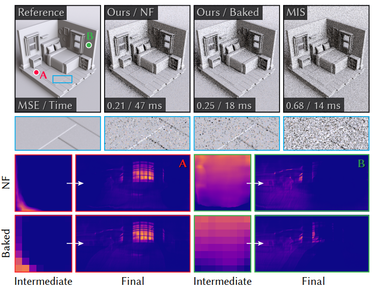
• 和 MIS、steaming RIS【ReSTIR DI】 相比，效果都不错【同时间】
  • MSE：0.111（MIS 0.224，RIS 0.148）

Microfacet materials

• distant emitter with a microfacet-based BRDF with a Trowbridge–Reitz (GGX) distribution
• 5D condition：surface normal、view direction、roughness
• 两种设置
  • rougness 为常数【0.2】：我们都是最优
  • roughness 从 【0.2-0.8】均匀采样：等时间比不过 RIS

Neural materials

• 和 NeuSample 类似，使用 NeuMIP 的特征向量表示
• 测试场景：three fabric materials with different glossiness
• 我们等时间最好

Shadow-catcher compositing

• 可以使用 shadow catcher method，往真实照片中插入虚拟物体
• 两个 pass
  • p1：inserted object + shadow catcher
  • p2：shadow catcher

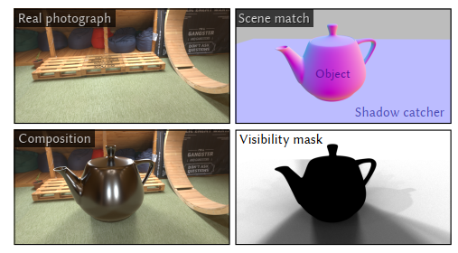
• 计算 p1/p2，shadow catcher 上 luminance 的比值，作为 visibility mask
  • 用于物体和真实照片的 alpha blending
• Lambertian shadow catcher：期望透明度
  • \(L\)：环境光源的 DI

\[ \tau = \frac{\int_{\Omega} V(\mathbf{x}, \omega) L(\omega) \langle \mathbf{n}, \omega \rangle \,\mathrm{d}\omega}{\int_{\Omega} L(\omega) \langle \mathbf{n}, \omega \rangle \,\mathrm{d}\omega}\tag{13} \]

• 如何一次 pass 估计？
• 等价于 \(V(\mathbf{x}, \omega)\) 的期望，分布为 \(L(\omega) \langle \mathbf{n}, \omega \rangle \Big/\int_{\Omega} L(\omega) \langle \mathbf{n}, \omega \rangle \,\mathrm{d}\omega\)

\[ \langle \tau \rangle_N = \frac{1}{N} \sum_{i=1}^{N} V(\mathbf{x}, \omega_i),\quad \omega_i \sim p_{\mathcal{X}}(\omega \vert \mathbf{x}; \theta) \tag{14} \]

• 加入物体：使用 visibility mask 做 alpha-blending
• 实验：真实图片是从环境光中提取出来的，同时获取相机位置【使用 fSpy】

Discussion

• 我们方法比直接使用 NF 近似分布好【大小相似】
• Ablation

• Limitations
  • 我们的模型需要 training per material model【单材质训练+光源是环境光，所以不需要考虑位置】
  • 材质粗糙度很小的时候【大头在 BSDF 支配】，head warp 效果不好
  • sun env 效果很差，tail 退化为点，不利于 head 优化
  • MIS 会引入额外 1 pass 网络推理开销