(论文)[2025-EGSR] Neural Path Guiding with Distribution Factorization
Neural Path Guiding with Distribution Factorization
- 作者:Pedro Figueiredo、Qihao He、Nima Khademi Kalantari
- Texas A&M University
- 之前的 PG 方法只占了一点【快、表达能力好】,我们试图又快又好
- 将 2D 分布拆分为两个 1D 的条件分布【神经网络输出1D 数组作为离散分布】
- 训练的时候,使用另外一个网络缓存 \(L_i\) 作为真值训练
Related Work
Global Path Guiding
- primary sample space(PSS)
- curse of dimensions、长路径表现差
- 偏镜面光路算法:specular chains 那一套
Local Path Guiding
- 空间、方向数据结构:kdtree、octree、vmf
- neural
- 近似分布参数、normalizing flow【问题在于表达能力不够】
- 基于 CNN,甚至只能在第一跳 pg【慢】
Radiance Caching
Histogram Prediction
Method
- 渲染方程
\[ L_o(\mathbf{x}, \omega_o) = L_e(\mathbf{x}, \omega_o) + \int_{\Omega} \rho(\mathbf{x}, \omega_o, \omega) L_i(\mathbf{x}, \omega) \lvert \cos(\theta) \rvert \,\mathrm{d}\omega \tag{1} \]
- pg 目的
- \(\Theta\) 表示 NN
\[ \hat{p}_{\Theta}(\omega \vert \mathbf{x}, \omega_o) \propto \rho(\mathbf{x}, \omega_o, \omega) L_i(\mathbf{x}, \omega) \vert \cos(\theta) \vert \]
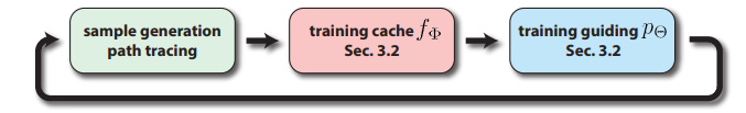
- pipeline
Distribution Factorization
- 需求
- 分布正比于目标分布
- 快速采样、计算 pdf
- 转换
- \(\phi=2\pi\epsilon_1,\theta=\arccos(1-2\epsilon_2)\)
- \(\hat{p}(\omega \vert \mathbf{x},
\omega_o)\) 可以转化为 \(\hat{p}(\epsilon_1, \epsilon_2 \vert \mathbf{x},
\omega_o)\)
- 需要考虑 Jacobian 矩阵
- 直接网络输出离散化的值【\(M_1\times M_2\)】 开销太大
- 拆分
- 如此只需要两个独立的网络分别输出 \(M_1\) 维的向量 \(\mathbf{v}_1\)、\(M_2\) 维的向量 \(\mathbf{v}_2\) 即可
\[ \hat{p}_{\Theta}(\epsilon_1, \epsilon_2 \vert \mathbf{x}, \omega_o) = \hat{p}_{\mathbf{w}_1}(\epsilon_1 \vert \mathbf{x}, \omega_o) \, \hat{p}_{\mathbf{w}_2}(\epsilon_2 \vert \epsilon_1, \mathbf{x}, \omega_o) \tag{3} \]
- 如何使用离散向量:nearest neighbor、linear
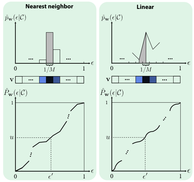
nearest neighbor
- \(\mathcal{C}\) 是条件的简记,忽略 \(\mathbf{v}\) 的下标【二者类似】
\[ \hat{p}_{\mathbf{w}}(\epsilon \vert \mathcal{C}) = \mathbf{v}[\lfloor\epsilon M\rfloor] \tag{4} \]
- cdf
\[ \hat{P}_{\mathbf{w}}(1) = \int_{0}^{1} \hat{p}_{\mathbf{w}}(\epsilon \vert \mathcal{C}) \,\mathrm{d}\epsilon = \sum_{i=0}^{M-1} \mathbf{v}[i] \frac{1}{M} = 1 \tag{5} \]
- 需要网络输出的向量 \(\mathbf{v}\)
和为 \(M\)
- 输出:softmax 归一化;乘上 \(M\)
- 采样:算出 cdf,然后用它的逆
linear
- 类似的,只不过 \(\mathbf{v}[i]\) 表示区间的中间值,然后剩余值插值【更平滑】
\[ \begin{align} \hat{p}_{\mathbf{w}}(\epsilon \vert \mathcal{C}) &= (1 - \alpha) \, \mathbf{v}[\lfloor m\rfloor] + \alpha \, \mathbf{v}[\lceil m\rceil] \tag{7} \\ \\ \text{where }&m = \epsilon M - 0.5,\alpha = m - \lfloor m \rfloor \tag{8} \end{align} \]
- cdf
\[ \hat{P}_{\mathbf{w}}(1) = \int_{0}^{1} \hat{p}_{\mathbf{w}}(\epsilon \vert \mathcal{C}) \,\mathrm{d}\epsilon = \sum_{i=0}^{M-1} \frac{\mathbf{v}[i] + \mathbf{v}[i+1]}{2} \cdot \frac{1}{M} = 1 \tag{9} \]
- 边界处理:\(\epsilon<\dfrac{1}{2M},\epsilon>1-\dfrac{1}{2M}\)
- \(\epsilon_1\)(\(\phi\)):对 \(\mathbf{v}_1[0],\mathbf{v}_1[M-1]\) 线性插值【\(0=2\pi\)】
- \(\epsilon_2\)(\(\theta\)):最近邻
- 两种处理结果都是正确的
- 中间部分 pdf 求和是:\(1-\dfrac{\mathbf{v}[0] + \mathbf{v}[M-1]}{2}\)
- 采样类似
Connection to NIS
- NIS 使用 normalizing flow 变换分布;而我们直接拆分后估计分布【离散向量】
Optimization with Radiance Caching
- NPM 训练使用 MC 的结果,我们使用 NN 缓存 incident radiance
- KL 散度估计【然后使用 MC 估计 KL 散度的积分】
- 理想目标分布
\[ p(\omega_i) = \underbrace{\rho(\mathbf{x}, \omega_o, \omega_i) L_i(\mathbf{x}, \omega_i) \vert \cos(\theta_i) \vert}_{\text{integrand}} \underbrace{L_r(\mathbf{x}, \omega_o)^{-1}}_{\text{normalization factor}} \tag{13} \]
- NPM 等实现
- \(L_i\) 使用 MC 估计【噪声大】
- \(L_r\) 忽略
- 如果针对一个 \(\mathbf{x}, \omega_o\) 进行训练是 ok 的
- 但是网络训练存在很多样本,这样会导致效果不好
- 使用 NRC(\(f_{\Phi}\))缓存 \(L_r\)【NRC 论文中明确说了缓存的就是 \(L_r\),所以和本文是一样的】
- 获取 \(L_i\)
\[ L_i(\mathbf{x}, \omega_i) = L_r(\mathbf{x}', \omega_o')=f_{\Phi}(\mathbf{x}', \omega_o') \]

- 同样 normalizing factor 也被解决了
- 实验效果上缓存 \(L_r\)
的效果比 \(L_i\) 更好
- 相当于过了一层 BSDF 的 filter
- 理论上这只是把方差从估计 KL 散度转移到了 NRC 上
- 但是效果确实很好
- 得益于估计 \(L_r\)、NRC 的高效实现【relative L2 loss】
- 和强化学习中的 actor-critic techniques 很像
- RL:缓存 reward,从而降低优化 policy 的噪声
Implementation
- Kiraray + TCNN
- 30% budget 用于训练
- 3 个网络:\(f_{\mathbf{w}_1}\)、\(f_{\mathbf{w}_2}\)、\(f_{\Phi}\)
- 70% guiding;30% BSDF
- \(M_1=32,M_2=16\)
Results
- NEE off,RR off
- max depth 6
- RTX 3080
- relMSE,去除 0.1% outlier,10 次取平均
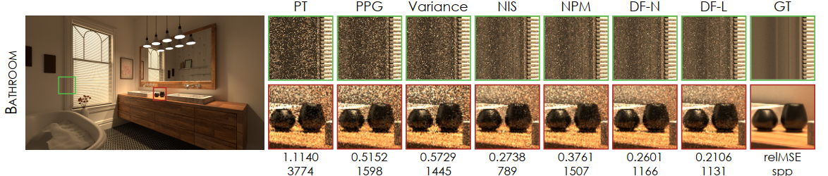
- 场景:小光源、光路难
- 对比算法
- PPG、Variance-Aware PG【估计 radiance】
- NIS、NPM、我们(DF-N、DF-L)【估计 product】
- We implement NIS with two fully-fused networks (L = 2) using piecewise quadratic coupling layers and fixed bin size and resolutions of 32 × 16 to match the capacity of our approach.
- 等时间比较【大概都是 DF-L 最优,DF-N 次优】
- 120s,30% 训练
- NIS 样本数更少【说明慢但是质量高】

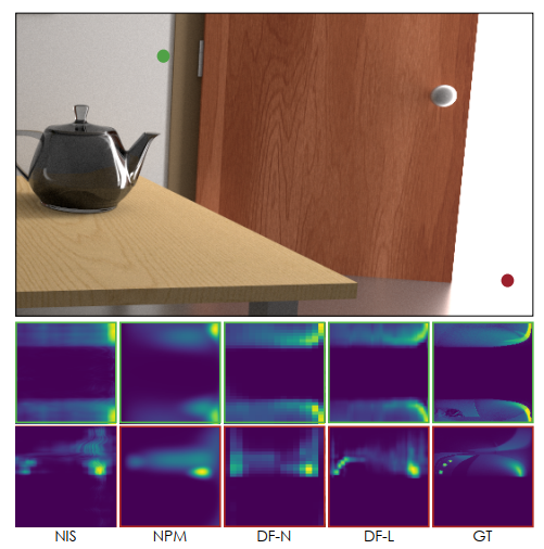
- 上面实验的分布好坏【这个例子设计的很难,6k spp PT
还是糊的不行】
- 只看了 product-based 的方法
- NIS 缺失细节,因为慢导致训练样本少
- NPM 糊了
- 收敛性分析
Ablation
- \(M_1,M_2\) 大小
- trade off:开销、质量
- caching \(L_r\),对比
- 式子中 \(L_i\) 用 MC 样本计算,\(L_r\) 忽略【No Cache】
- 式子中 \(L_i\) 用 \(L_r\) 计算,\(L_r\) 忽略【\(L_i\)】
- 式子中 \(L_i\) 用 \(L_r\) 计算,\(L_r\) 也用【\(L_i+L_r\)】
Future
- 网络直接估计可变的 \(M_1,M_2\)
- 局限
- pdf 不够 sharp:游泳池场景不能很好学到光源方向,比不上 PPG 传统方法
- 简单场景 PT、NPM 可能更好
- Futrue:把 NN 和显式数据结构结合