(论文)[2002-EG] A Simple and Robust Mutation Strategy for the Metropolis Light Transport Algorithm

Posted on 2025-03-21 Edited on 2025-04-07 In CG.Paper Views:

PSSMLT，将 MLT 的突变放到了 Primary Space，这样就不需要特地去设计变异策略；另外引入了 large step 的变异，同时保证了遍历性、高接收率、以及 MIS 的引入（优化了暗处）

PSSMLT

Primary Space Sample Metropolis Light Transport
MIS 部分是作者论文另外一个版本
简单实现：原版，备份

Introduction

\[ \Phi_{j}=\int_{\mathcal{P}} F(\mathbf{z})\,\mathrm{d}\mathbf{z} \approx \frac{1}{M}\sum_{i = 1}^{M}\frac{F(\mathbf{z}_i)}{p(\mathbf{z}_i)} \]

重要性采样：正比于分子
- 3d => 1d：scalar contribution function \(I(\mathbf{z})\)
  - 例如：luminance
- 于是：\(p(\mathbf{z})=I(\mathbf{z})/b=I(\mathbf{z})/\int_{\mathcal{P}} I(\mathbf{z})\,\mathrm{d}\mathbf{z}\)

Local and multiple importance sampling

primary space：\(\mathcal{U}\)
生成一条路径用的随机数：\(\mathbf{z}\in\mathcal{U}\)
路径：\(\mathbf{z}=S(\mathbf{u})\)
于是贡献值

\[ \Phi_{j}=\int_{\mathcal{U}} F(S(\mathbf{u}))\cdot\left|\frac{\mathrm{d}S(\mathbf{u})}{\mathrm{d}\mathbf{u}}\right|\,\mathrm{d}\mathbf{u} \]

Jacobian

\[ \left|\frac{\mathrm{d}S(\mathbf{u})}{\mathrm{d}\mathbf{u}}\right|=\dfrac{1}{p_S(\mathbf{u})} \]

如果 \(\mathbf{u}\) 是均匀分布，那么 \(p_S(\mathbf{u})\) 就是 \(\mathbf{z}=S(\mathbf{u})\) 的 pdf
随机决定当前 bounce 使用 light sampling/BSDF sampling 会导致目标函数不一样
- 加入 MIS

MLT

采样整条路路径，而不是一个方向
平稳分布 \(p(\mathbf{z})\)

对所有像素定义一个过程（one single process for all pixels）
- \(I\) 近似 radiance，和像素无关
- 这样直方图就对应像素的 luminance
存在 start-up bias
- 原始解决方案：\(p_0\) 生成一些样本，然后从这些样本中根据 scalar contribution function 重采样得到初始样本
新老样本都用，效果更好【\(a\bar{y}+(1-a)\bar{x}\)】
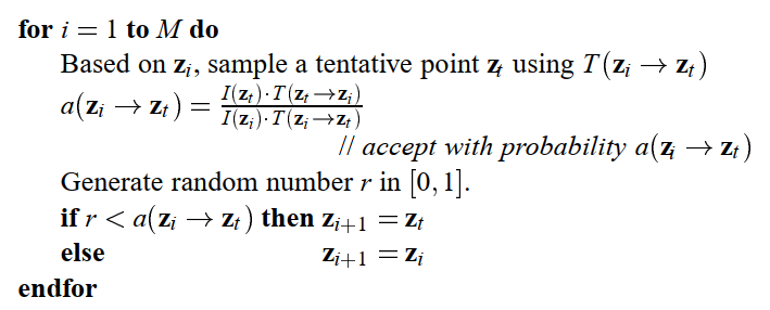
MLT 算法如下

MLT 生成的样本是相关的
MC 保证标准差 \(=\sigma_{\text{primary}}\Big/\sqrt{M\text{ samples}}\)
相关样本（Bernstein theorem）
- \(R(k)\) 表示样本 \(F(\mathbf{z}_i)/p(\mathbf{z}_i),F(\mathbf{z}_{i+k})/p(\mathbf{z}_{i+k})\) 相关性的上界
- 样本之间的相关性会导致 error 增加

\[ \sigma\le\sigma_{\text{primary}}\sqrt{\dfrac{1+2\sum_{k=1}^MR(k)}{M}} \]

小扰动导致相关性大大【独立机会小】
大扰动也可能导致大相关性【接受概率小】

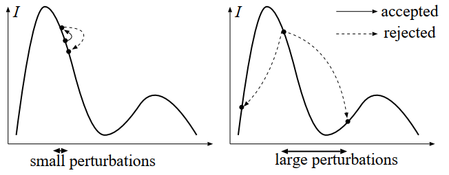
于是我们需要一种变异策略：一般情况来说变异大，积分值大的地方变异小
MLT 原始论文：设计了 3 种针对不同光路的变异策略，具体选择依赖于场景相关的超参
我们：简单的自动选择变异的策略

好的变异空间

如何实现上面说的积分值大的地方变异小？
- 变换到一个方差小的函数 \(f'\)，此时如果在这个函数中使用固定的变异步长，则其在原始空间中就实现了上面这一点
- 积分值大 => 对应到 \(f'\) 的更大范围
  - 于是相同的 \(f'\) 的范围，原始积分值大则对应小的范围，原始积分值小则对应大的范围
primary sample space
新的积分、scalar contribution function
- 方差小
- 例如 glossy lobe，随机数动一点，方向在 lobe 上的变化很小

\[ F^{*}(\mathbf{u}) = F(S(\mathbf{u}))\cdot\left|\frac{dS(\mathbf{u})}{d\mathbf{u}}\right|=\frac{F(S(\mathbf{u}))}{p_S(\mathbf{u})} \]

\[ I^{*}(\mathbf{u})=\frac{I(S(\mathbf{u}))}{p_S(\mathbf{u})} \]

PT 例子

直接光采样的例子【不够有效】
- \(u_1,u_2\)：选择一个像素位置
- \(u_3\)：选择一种 BRDF、是否 RR
- （继续 PT）\(u_4,u_5\)：采样反射方向
- \(u_6\)：RR 停止
- \(u_7,u_8\)：光源采样位置

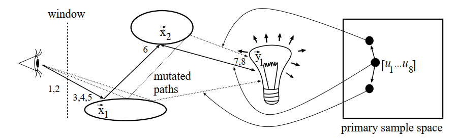
扰动如上图

BPDT 例子

eye path、light path：所有顶点连接测试可见性
- 下图实线表示 subpath
- 虚线表示连接

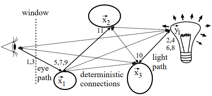
这里使用 maximum heuristic MIS
- 好处是不需要追完所有 shadow ray，如果不考虑可见性都不是最大就不用追了
一个 PSS 对应 BDPT 生成多条可行光路，需要重新定义 scalar contribution function
- 所有 path 的 luminance 之和【倾向生成长路径，计算开销大】
- 使用 path 的最大 luminance
  - 这最终只用了最大 luminance 的贡献？
如果 RR 导致 eye path 节点变少，此时下一个原本用于 eye path 的随机数会被用于 light path，造成剧烈变化
- 于是我们将两边生成位置的随机数分离；例如奇数用于 eye path，偶数用于 light path

Large step

MLT 需要遍历
很多光路贡献为 0，因此存在“距离”较远的区域，需要的大的变异才能满足遍历性
加上一种不考虑原始状态的变异方式，称为 large steps
好处
- 遍历性
- Metropolis 算法从新的种子开始，减小 start bias
- 样本 pdf 已知，可以用于后续的 MIS【？】
如何选择新样本？希望接收率大
- 新样本的概率与旧样本无关：\(T(\mathbf{z}_i\to\mathbf{z}_t)=T(\mathbf{z}_t)\)
- 如果 \(T\propto I\)，则 \(a=0\)；但是不可能实现

\[ a(\mathbf{z}_i\to\mathbf{z}_t)=\dfrac{I(\mathbf{z}_t)\cdot T(\mathbf{z}_i)}{I(\mathbf{z}_i)\cdot T(\mathbf{z}_t)} \]

primary space
- 实现的时候用的是这个版本，不管 larrge step 还是常规变异 \(T_x=T_y\) 都相同

\[ a(\mathbf{u}_i \rightarrow \mathbf{u}_t)=\frac{I^{*}(\mathbf{u}_t)\cdot T^{*}(\mathbf{u}_i)}{I^{*}(\mathbf{u}_i)\cdot T^{*}(\mathbf{u}_t)} \]

将 \(I^{\ast}\) 近似为常数【低方差】

\[ a(\mathbf{u}_i \rightarrow \mathbf{u}_t)\approx\frac{ T^{*}(\mathbf{u}_i)}{T^{*}(\mathbf{u}_t)} \]

此时，如果变异策略是随机采样，则接受率近似为 1

变异策略

Designing mutation strategies in the infinite dimensional cube：lazy evaluation
空间是无限的，如何变异
如果一个变量 \(u\) 没有被用到，那么就不需要更新它【不用每次都更新他，用的时候再更新】
具体看第 6 章节的实现部分

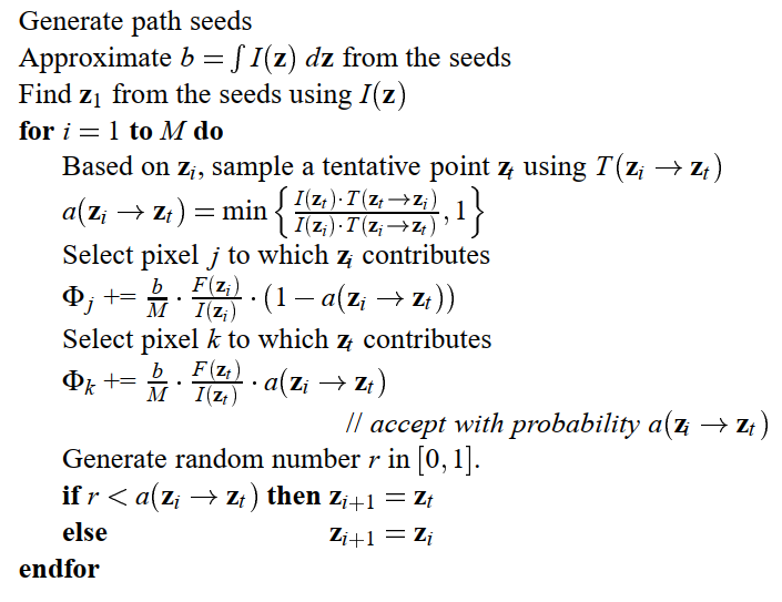
Utilization of rejected and large step samples

原始 MLT 利用被拒绝样本的方式：记录他们的加权均值
large step sample 能用 MIS 更好处理
MLT 通过 \(p_1(\mathbf{u})\) 生成 \(M_1\) 个样本；large step 通过 \(p_2(\mathbf{u})\) 生成 \(M_2\) 个样本
balance heuristic MIS

\[ \begin{aligned} w_1(\mathbf{u}) = \frac{M_1 p_1(\mathbf{u})}{M_1 p_1(\mathbf{u}) + M_2 p_2(\mathbf{u})}\\ w_2(\mathbf{u}) = \frac{M_2 p_2(\mathbf{u})}{M_1 p_1(\mathbf{u}) + M_2 p_2(\mathbf{u})} \end{aligned} \]

MLT：\(p_1(\mathbf{u})=I^{\ast}(\mathbf{u})/b\)
large step：\(p_2(\mathbf{u})=1\)
如果 \(p_{\text{large}}\) 表示采样 large step 的概率
- \(M_1=M\rightarrow M_2=p_{\text{large}}M\)【一共变异 \(M\) 次，large step 的时候同时生成两个样本】

\[ M_1 p_1(\mathbf{u}) + M_2 p_2(\mathbf{u})=M(I^{\ast}(\mathbf{u})/b+p_{\text{large}}) \]

\[ w_1(\mathbf{u})= \frac{I^{\ast}(\mathbf{u})/b}{I^{\ast}(\mathbf{u})/b+p_{\text{large}}} \]

\[ w_2(\mathbf{u})= \frac{p_{\text{large}}}{I^{\ast}(\mathbf{u})/b+p_{\text{large}}} \]

加权
旧样本的贡献【MLT 转移成功，但是使用加权贡献】
- 其实都一样了，\(w\) 和 \(F/p\) 的 \(p\) 消掉了
- 转移失败 \((1-a)\) 就是 \(1\) 了

\[ (1 - a)\cdot w_1(\mathbf{u})\cdot \dfrac{F^{*}(\mathbf{u})}{p_1(\mathbf{u})}=\frac{(1 - a)}{I^{*}(\mathbf{u})/b + p_{\text{large}}}\cdot F^{*}(\mathbf{u}) \]

新样本的贡献（large step）
- the generated path is a sample of the Metropolis method and a sample of the uncorrelated strategy at the same time【贡献两次】
  - 怎么理解这个既是又是：相当于在原来的整体估计上，叠加上了一个无偏估计，是正确的【因为反正是直方图】
- 然后 MLT 部分需要被加权

\[ a\cdot w_{1}(\mathbf{u})\cdot \dfrac{F^{*}(\mathbf{u})}{p_1(\mathbf{u})} + w_{2}(\mathbf{u})\cdot \dfrac{F^{*}(\mathbf{u})}{p_2(\mathbf{u})}=\frac{(a + 1)}{I^{*}(\mathbf{u})/b + p_{\text{large}}}\cdot F^{*}(\mathbf{u}) \]

新样本的贡献（small step）

\[ a\cdot w_1(\mathbf{u})\cdot \dfrac{F^{*}(\mathbf{u})}{p_1(\mathbf{u})}=\frac{a}{I^{*}(\mathbf{u})/b + p_{\text{large}}}\cdot F^{*}(\mathbf{u}) \]

使用变量 \(\text{large-step}\) （0，1）统一表示两个式子

\[ \frac{(a+\text{large-step})}{I^{*}(\mathbf{u})/b + p_{\text{large}}}\cdot F^{*}(\mathbf{u}) \]

理解：large step 和 MLT 做 MIS；然后 MLT 使用 \((a,1-a)\) 加权

实现理解

mitsuba0.6 的实现，把所有权重都乘上了 \(I^{*}(\mathbf{u})\)，但是在 Veach-Style 用的还是 \((a,1-a)\)【没乘】
实现需要这样，实验

讨论

如果是灰度图，那么每个样本累计 1，最终的直方图就是灰度的分布
- 和下面的 Veach-Style 一样，这里是以 \(a\) 概率累计 \(I_{\text{new}}\)，\(1-a\) 概率累计 \(I_{\text{old}}\)
- 而 Veach-Style 直接累计 \(aI_{\text{new}}+(1-a)I_{\text{old}}\)
- 表达式是一样的
如果是颜色图，那么每个样本累计用 \(I(\cdot)\) 归一化之后的 color 值
- 使用 \(I(\cdot)\) 作为平稳分布，那么得到的结果就已经是 \(I(\cdot)\) 的一个近似了；在其上面乘上平均颜色就是结果
- \(I(\cdot)\) 一般使用 luminance
Veach-Style 理解
- 这里还是分布，相当于累积到直方图（图片上）的值需要正比于 \(I(\cdot)\)
- 权重只能是 \((a,1-a)\)，试过 \((0.5,0.5)\) 结果是错的，具体理解如下
- 假设灰度；假设目前达到了平稳分布 \(p\)
  - 灰度转化为 color，和上面颜色的转化一样
- 那么累积到像素 \(i\) 的期望贡献如下，于是累计的时候累计的 \(I_i=1\)（注意到推导过程没有用到 \(I_i\) 信息，所以可以这么搞），此时便正比于 \(p_i\) 了

\[ \begin{aligned} &p_i\left(\sum_{j\ne i} T_{i\to j}\left(1-a_{i\to j}\right)I_{i}\right)+\sum_{j\ne i} p_j\left(T_{j\to i}a_{j\to i}\right)I_{i}\\ =&\sum_{j\ne i}\left( p_iT_{i\to j}\left(1-a_{i\to j}\right)+ p_jT_{j\to i}a_{j\to i}\right)I_{i}\\ =&\sum_{j\ne i}\left( p_iT_{i\to j}- p_iT_{i\to j}a_{i\to j}+ p_jT_{j\to i}a_{j\to i}\right)I_{i}\\ (细致平衡)=&\sum_{j\ne i}\left( p_iT_{i\to j}\right)I_{i}\\ =&p_iI_i \end{aligned} \]

Kelemen-Style 理解
- 最终累积到图片上的就是和 PT 一样估计的最终结果
  - 然而此时的 color 已经被 \(I(\cdot)\) 归一化了，因此需要乘回去
- 这是一种重要性采样，假设我们现在已经达到了细致平衡
- 计算得到的权重就是最终两种采样方式的 MIS 权重
- 两种方式都用，相当于在最终结果上再叠加了一层 PT 的结果，所以也是对的
- proposedWeight 这一部分 (a + (largeStep ? 1 : 0)) 修改为我们认知中的 (largeStep ? a : 1) 当然也是正确的
  - 这样的话相当于就是 1 个样本

if (a > 0) {
    if (m_config.kelemenStyleWeights && !m_config.importanceMap) {
        /* Kelemen-style MLT weights (these don't work for 2-stage MLT) */
        currentWeight = (1 - a) * current->luminance
            / (current->luminance/m_config.luminance + m_config.pLarge);
        proposedWeight = (a + (largeStep ? 1 : 0)) * proposed->luminance
            / (proposed->luminance/m_config.luminance + m_config.pLarge);
    } else {
        /* Veach-style use of expectations */
        currentWeight = 1-a;
        proposedWeight = a;
    }
    accept = (a == 1) || (random->nextFloat() < a);
} else {
    if (m_config.kelemenStyleWeights){
        currentWeight = current->luminance
            / (current->luminance/m_config.luminance + m_config.pLarge);
    }
    else {
        currentWeight = 1;   
    }
    // ...
}

实现细节

mitsuba0.6 上的实现似乎和文章是一样的，看看代码
PrimarySample(i)，生成第 \(i\) 个随机数
- 布尔变量 \(\text{large-step}\)
- push 是保存旧的状态，如果被拒绝了的话，用于恢复旧的样本

float PrimarySample(int i) {
    if (u[i].modify < time) {
        if (large_step) { // large step
            Push(i, u[i]); // save state
            u[i].modify = time;
            u[i].value = random();
        } else { // small step
            if (u[i].modify < large_step_time) {
                // large step 之后就和之前独立了，因此只需要记录最新的 large_step_time
                u[i].modify = large_step_time;
                u[i].value = random();
            }
            // lazy evaluation of mutations
            while (u[i].modify < time-1) {
                u[i].value = Mutate(u[i].value);
                u[i].modify++;
            }
            Push(i, u[i]); // save state
            u[i].value = Mutate(u[i].value);
            u[i].modify++;
        }
    }
    return u[i].value;
}

变异策略：\([s_1,s_2]\) 之间

float Mutate( float value ) {
    float s1 = 1./1024, s2 = 1./64;
    float dv = s2*exp(-log(s2/s1)*random());
    if (random() < 0.5) {
        value += dv; if (value > 1) value -= 1;
    } else {
        value -= dv; if (value < 0) value += 1;
    }
    return value;
}

每个样本至少会贡献两次（刚生成，新的生成而且被接受）
- Next 函数返回失效样本，保留还在用的样本
- 直接把贡献权重累计
- contrib: \(F^{\ast}(\mathbf{u})\)
  - 可能是个数组，贡献给多个像素
- I：\(I^{\ast}(\mathbf{u})\)
- 接收率计算不需要考虑转移函数 \(T\)，因为不管是 large/small，\(T\) 都是对称的

Sample Next(float I, Contrib contrib) {
    float a = min(1, I/oldI); // accept prob.
    newsample.contrib = contrib;
    newsample.w = (a+large_step)/(I/b+plarge)/M;
    // cumulate weight
    oldsample.w += (1-a)/(oldI/b+plarge)/M;
    if (random() < a) { // accept
        oldI = I;
        contribsample = oldsample;
        oldsample = newsample;
        if (large_step) large_step_time = time;
        time++;
        ClearStack(); // no state restoration
    } else { // reject
        contribsample = newsample;
        // restore state
        while( !IsStackEmpty() ) Pop(i, u[i]);
    }
    large_step = (random() < plarge) ? 1 : 0;
    return contribsample;
}

Evaluation

pt，simple BDPT（只连端点）、normal BDPT（所有点都连）
MLT 只改动局部，获取样本计算代价小；我们需要重新构建，计算代价大
- 需要同时间比较
验证了我们算法的有效性、MIS 的有效性

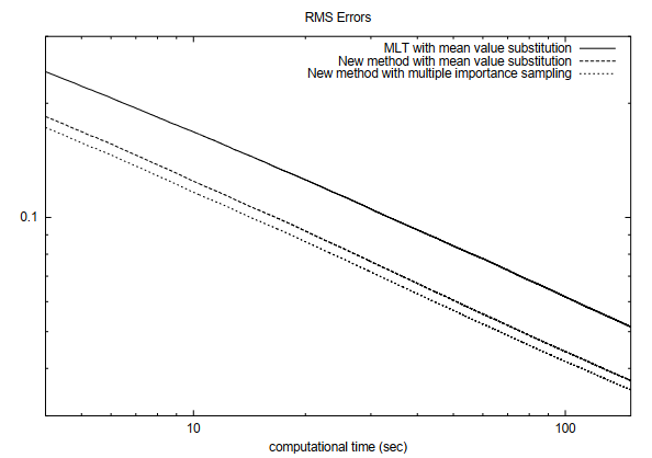
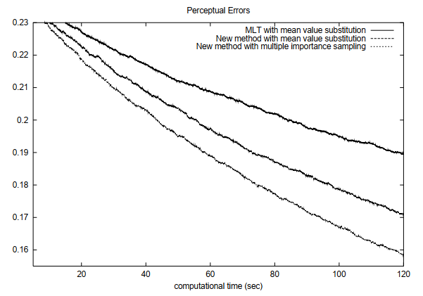
复杂场景 MIS 效果好
- 尤其是复杂场景的暗处【MLT 本身处理暗处效果不好】
large step 降低相关性带来的 bias