(论文)[2024-SIGA-C] MARS: Multi-sample Allocation through Russian roulette and Splitting
MARS
- 项目主页
- 作者
- JOSHUA MEYER, ALEXANDER RATH(EARS 一作), ÖMERCAN
YAZICI
- Saarland University, Germany
- PHILIPP SLUSALLEK, German Research Center for Artificial Intelligence, Germany and Saarland University, Germany
- JOSHUA MEYER, ALEXANDER RATH(EARS 一作), ÖMERCAN
YAZICI
- mitsuba 0.6
Introduction
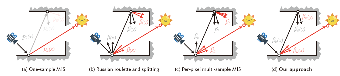
在之前的算法,MIS 一般都只考虑 1 sample MIS,而 RRS 工作中,对于每个 N,选择相同数量的 NEE、BSDF 光线
本文优化了这点,MIS 的时候,不同策略自动选择最优的光线数
示意图
- 只和像素有关
- 和像素、位置都相关
之前工作
- Importance sampling (IS)(path guiding)
- Multiple importance sampling(MIS)
- Path tracing
- Bidirectional methods:BDPT
- 每个视子路连接相同数量的光子路
- Mixture sampling ratios
- 大部分只考虑直接光照,也就是说,这个 MIS weight 是 per-pixel 的【上图 (c)】
- 只优化了:one-sample MIS
- Russian roulette and splitting
- BSDF rays 的数量和 NEE rays 相同
- Multi-sample allocation
- 简单 RRS + MIS ratio 效果不好,应该被联合优化
理论
- 不动点迭代,EARS 的推导泛化
\[ I=\int_{\mathcal{X}}f(x)\,\mathrm{d}x \]
- model
- \(n_t\) 种采样策略,策略 \(t\) 分配 \(\beta_t\) 条光线(budget)
- \(\langle I_t\rangle\):primary estimator of technique \(t\)
- \(\langle I;\beta\rangle\):secondary estimator for \(I\) with \(\beta\) samples
\[ \langle I\rangle=\sum_{t=1}^{n_{t}}{\frac{1}{\beta_{t}}}\sum_{s=1}^{\beta_{t}}\langle I_{t}(x_{t,s})\rangle=\sum_{t=1}^{n_{t}}\langle I_{t}(x_{t},\cdot);\beta_{t}\rangle \]
- 不同策略定义域可能不同(总的定义域需要包含整体),需要计算权重
\[ \langle I_{t}(x)\rangle=\sum_{i=1}^{n_{i}}{\frac{f_{i}(x)}{p_{t}(x)}}w_{i t}(x) \]
- 连续样本数:\(\beta_t\in\mathbb{N}\to\mathbb{R}^{+}\)(好操作),最终计算光线数
\[ r(\beta)= \left\{ \begin{array}{l l} \lfloor\beta\rfloor+1&\quad\text{with probability }\beta-\lfloor\beta\rfloor,\\ \lfloor\beta\rfloor&\quad\mathrm{otherwise}\\ \end{array} \right. \]
- 效率
\[ {\mathcal{E}}\left[\langle I\rangle\right]=\frac{1}{\mathbb{V}\left[\langle I\rangle\right]\mathbb{C}\left[\langle I\rangle\right]} \]
- 需要考虑每一个样本 \(\beta_t\) 的 variance 和 cost
cost model
- 每种策略的代价求和 + 汇总的代价 \(\mathbb{C}_{\Delta}\)
\[ \mathbb{C}\left[\langle I\rangle\right]=\sum_{t=1}^{n_t}\beta_t\mathbb{C}_t+\mathbb{C}_{\Delta} \]
variance model
- 首先对所有独立采样策略求和
- 【式子 1】
\[ \mathbb{V}\left[\langle I\rangle\right]=\sum_{t=1}^{n_t}\mathbb{V}\left[\langle I_{t};\beta_{t}\rangle\right] \]
- 存在 stochastic rounding(小数部分)【先不管,副录有证明】
- \(\langle I_t\rangle\) 表示只用这种技术(的方差、期望)
\[ \mathbb{V}\left[\langle I_{t};\beta_{t}\rangle\right] = \frac{1}{\beta_{t}}\mathbb{V}\left[\langle I_{t}\rangle\right] + \rho(\beta_{t})\mathbb{E}^{2}\left[\langle I_{t}\rangle\right] \]
\[ \rho(\beta)=\dfrac{(\beta-\lfloor\beta\rfloor)(\lceil\beta\rceil-\beta)}{\beta^2} \]
优化
- 找到最优的 \(\beta_t\),让 \({\mathcal{E}}^{-1}\left[\langle I\rangle\right]\) 最小
- 方差计算
- 推导
- 但是由于 \(\beta_t>1\)
的时候,存在 stochastic rounding,这里有近似
- 近似:把复杂的 \(\rho(\beta)\) 不管了
- EARS 也使用了这种近似
- 近似:把复杂的 \(\rho(\beta)\) 不管了
- \(\beta_t\le 1\) 不存在近似的
- 【式子 2】
\[ \mathbb{V}\left[\langle I_t;\beta_t\rangle\right]= \left\{ \begin{array}{ll} \dfrac{1}{\beta_t}\mathbb{E}\left[\langle I_{t}\rangle^2\right]-\mathbb{E}^2\left[\langle I_{t}\rangle\right]&\text{if }\beta_t\le1 \\ \dfrac{1}{\beta_t}\mathbb{V}\left[\langle I_{t}\rangle\right]&\text{otherwise}\\ \end{array} \right. \]
proxy model
\[ \dfrac{\mathrm{d}\mathbb{V}\left[\langle I\rangle\right]}{\mathrm{d}\beta_t}= \left\{ \begin{array}{ll} -\dfrac{1}{\beta_t^2}\mathbb{E}\left[\langle I_{t}\rangle^2\right]+\sum_{k=1}^{n_t}\dfrac{1}{\beta_t}\dfrac{\mathrm{d}\mathbb{E}\left[\langle I_{k}\rangle^2\right]}{\mathrm{d}\beta_t}&\text{if }\beta_t\le1 \\ -\dfrac{1}{\beta_t^2}\mathbb{V}\left[\langle I_{t}\rangle\right]+\sum_{k=1}^{n_t}\dfrac{1}{\beta_t}\dfrac{\mathrm{d}\mathbb{V}\left[\langle I_{k}\rangle\right]}{\mathrm{d}\beta_t}&\text{otherwise}\\ \end{array} \right. \]
- MIS 权重会存在 \(\beta_t\),所以第二项很难计算
- 论文只考虑 balance heuristic
- 对于 budget-unaware MIS weights(MIS 权重不包含 \(\beta_t\)),第二项为 0,可以化简如下
\[ \dfrac{\mathrm{d}\mathbb{V}\left[\langle I\rangle\right]}{\mathrm{d}\beta_t}= \left\{ \begin{array}{ll} -\dfrac{1}{\beta_t^2}\mathbb{E}\left[\langle I_{t}\rangle^2\right]&\text{if }\beta_t\le1 \\ -\dfrac{1}{\beta_t^2}\mathbb{V}\left[\langle I_{t}\rangle\right]&\text{otherwise}\\ \end{array} \right. \]
- 上述 proxy 是 bugdet-unware MIS 最优的
- 如果是 budget-aware MIS,可能会偏离最优解
- 做了两个实验说明问题,说明不考虑上面的第二项时,会出现问题
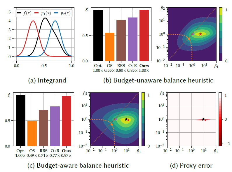
- 差别不大(1D、实验)
- 在应用中(PG、BDPT),比理论最优解更好
- 做了两个实验说明问题,说明不考虑上面的第二项时,会出现问题
- 下图是 1D 实验
- 积分函数 \(f(x)\)
- 两个采样 pdf \(p_1(x),p_2(x)\)
- \(p_2\) 更好,但是慢 30x
- 方法:OS(Optimal mixture
sampling)、RRS、OS+RRS、Ours、Opt(理论最优)
- OS+RRS 效果并不好,因为没有联合优化
- (b)(c)热力图应该是表示 performance
- (d)表示 (c) 中考虑/不考虑 MIS 中含有 \(\beta_t\) 的梯度 error(1 表示完全匹配)
不动点
- 推导方式和 EARS 基本一致,结论也看着差不多
- 【先不管,副录有证明】
\[ \beta_t= \left\{ \begin{array}{ll} \beta_{t}^{\mathrm{RR}}=\sqrt{ \dfrac{\mathbb{C}\left[\langle{I}\rangle\right]} {\mathbb{C}_t} \dfrac{\mathbb{E}\left[\langle{I_t}\rangle^2\right]} {\mathbb{V}\left[\langle{I}\rangle\right]}} &\text{if }\beta^{\text{RR}}<1 \\ \beta_{t}^{\mathrm{RR}}=\sqrt{ \dfrac{\mathbb{C}\left[\langle{I}\rangle\right]} {\mathbb{C}_t} \dfrac{\mathbb{V}\left[\langle{I_t}\rangle\right]} {\mathbb{V}\left[\langle{I}\rangle\right]}} &\text{if }\beta^{\text{S}}>1 \\ 1&\text{otherwise} \end{array} \right. \]
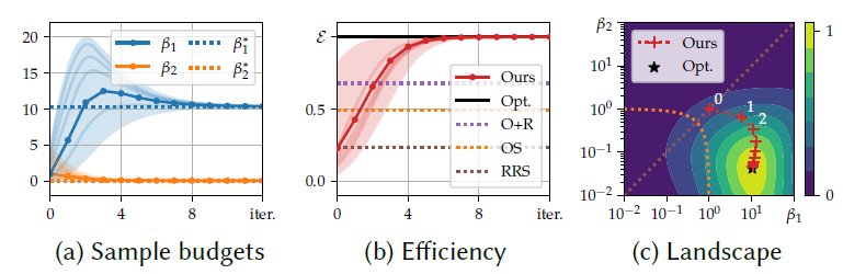
- 解析解难算,使用不动点迭代求解
- 收敛快,上面 1D 例子
Application to Path Tracing
- Primary estimator
\[ \langle L_{\text{r},t}(x,\omega_{0})\rangle=\frac{\langle L_{\mathrm{i}}(x,\omega_{\mathrm{i}})\rangle\,B(x,\omega_{\mathrm{i}},\omega_{0})\left|\cos\theta_{\mathrm{i}}\right|}{p_t(\omega_{\mathrm{i}}\mid x,\omega_{0})}\;w_{t}(x,\omega_{\mathrm{i}},\omega_{\mathrm{o}}), \]
- Secondary estimator
- path prefix \(\bar{x}\)
\[ \langle L_\text{r}(x,\omega_{0})\rangle=\sum_{t=1}^{n_{t}}\frac{1}{\beta_{t}(\bar{x})}\sum_{s=1}^{\beta_{t}(\bar{x})}\langle L_{\text{r},t}(x_{s},\omega_{0})\rangle=\sum_{t=1}^{n_{t}}\langle L_{\text{r},t};\beta_{t}(\bar{x})\rangle \]
- Random walks(PT 过程),递归
- 效率定义:EARS 相同,var 使用 \(I_{\text{px}}^2\) 归一化
- 优化:和上面类似
\[ \beta_t= \left\{ \begin{array}{ll} \beta_{t}^{\mathrm{RR}}= \dfrac{T(\bar{x})}{I_{\text{px}}} \sqrt{ \dfrac{\mathbb{C}_{\mathrm{I}}} {\mathbb{C}_t} \dfrac{\mathbb{E}\left[\langle{L_{\text{r},t}}\rangle^2\right]} {\mathbb{V}_\mathrm{I}}} &\text{if }\beta^{\text{RR}}<1 \\ \beta_{t}^{\mathrm{RR}}=\sqrt{ \dfrac{\mathbb{C}_{\mathrm{I}}} {\mathbb{C}_t} \dfrac{\mathbb{V}\left[\langle{L_{\text{r},t}}\rangle\right]} {\mathbb{V}_\mathrm{I}}} &\text{if }\beta^{\text{S}}>1 \\ 1&\text{otherwise} \end{array} \right. \]
- \(T(\bar{x})\):累乘
- 相机响应函数、\(1/\text{pdf}\)、BSDF、MIS 权重
应用1-Path Guiding
- NEE + BSDF + PPG
- 基本上和 EARS 一样
- PPG 的一轮迭代,认为是我们的一轮不动点迭代
- local estimates
- cost, variances, and second moments for each region and each technique
- image statistics:OIDN denoiser
- Fixed-point iteration
- warm up:前 3 轮,throughput based RR + no Splitting
- outlier clampling
- 路径贡献 clamp <= 50 pixels color【只用于 local/image variance 估计】
- \(\beta_t\):[0.05, 20]
- Handling colors:channel-wise 计算,然后乘在一起
- perform computations channel-wise and use the \(L_2\) norm to compute the final sample counts【啥意思?】
Evaluation
- path guiding:based on mixture optimization using gradient descent【Vorba et al. 2019】
- EARS
- 对比:throughput-based RR【5th bounce 开始】
- 其他:1st bounce 开始
- An ablation (“Ours + Grad. Descent”)【TODO】
- combines gradientdescent (mixing BSDF and guiding) and our approach (sample counts of NEE and the mixture) to demonstrate that our approach chooses better mixtures than the previous state-of-the-art optimizer.
- setup
- 2.5min训练+2.5min测试
- maxpath length:40
- tree:72MB
- 9 training iterations:time x2
- relMSE 评估
- 1% brightest outliers removal
- 十个场景:1.32× 加速(相对 EARS)、17% fewer rays
- 讲道理应该和 EARS+Optimal MIS 对比才有说服力
- 我们的方法能够检测在不同的点,什么方法更差【然后降低他的采样数】
- 收敛测试:我们算法能收敛到正确解
应用2-BDPT
- 【略过,不太懂】
限制与展望
- overhead:短时间训练,收集的统计信息不好,结果不好
- Local estimates:outlier removal 太简单,参考更复杂的
- 【EG-2018】Re-Weighting Firefly Samples for Improved Finite-Sample Monte Carlo Estimates
- Discontinuity artefacts
- Noise in the spatial caches
- Proxy accuracy
- Dynamic scenes
- MIS weights:只考虑了平衡启发式
- Correlated Techniques
- 方差拆分认为是独立的,没有考虑相关的情况(photon mapping)
- Applications outside of rendering
- any Monte Carlo integration problem that relies on multi-sample MIS estimation