(论文)[2024-SIGA] BSDF importance sampling using a diffusion model
BSDF importance sampling using a diffusion model
- 项目主页
- 作者:Ziyang Fu, Yash Belhe, Haolin Lu, Liwen
Wu, Bing Xu, Tzu-Mao Li
- University of California San Diego
- 引入了 diffusion 的神经采样,离线训练(3-3.5h)、实时推理(50ms pytorch、5ms vulkan)
摘要
- 之前的神经采样方法:解析的 lobe mixtures、归一化流(normalizing
flows)
- 很难处理 specular 材质(尤其是 grazing angle)
- 限制在反射上(不能处理折射)
- 归一化流为了保持好算的 Jacobian,加了很多限制
- 但是对于低维的 BSDF 采样,Jacobian 不难算
- 我们引入了扩散模型(deterministic diffusion model)
- 算法变种
- 针对大多数反射材质:learns a distribution on a disk
- extremely specular reflective materials and full BSDFs:learns a distribution on a sphere
- 同时间比较比之前方法好
Introduction
- BSDF
- 解析的 BSDF 有好的采样方法,但是不能真实模拟细节
- 打表的方式效果真实,但是需要大量存储开销
- NN 压缩 BSDF
- 但是他们都没有很好的采样的方式(sampling routine)
- NeuSample:【2023-SIGC】,处理反射
- 两种方案
- 使用 NN 预测 a mixture of Gaussian lobes
- normalizing flows(原论文认为这个最准,但是为了方便计算 Jacobian 加上了很多限制)
- 两种方案
- 引入:deterministic diffusion model
- 出发点:Jacobian 计算不是瓶颈
- 作用如同 ordinary differential equation (ODE) integrator,进行 sampling transformation
- 保证表达能力的同时,可微+双射
- RTX4090,1024x1024,4spp,60fps
- 贡献
- 同速度下,比归一化流表达能力更强;复杂分布下,比其更准
- 能处理折射
- 针对不同的材质设计不同方法
- diffuse:projected hemisphere domain
- glossy/specular:spherical domain
Related Work
- BSDF representation and compression
- tabulated BSDF measurements
- analytical BSDF models
- neural representations
- RGL material dataset 上测试
- BSDF Importance sampling
- tabular solutions
- fitted parametric analytical models
- a parametric Blinn-Phong model
- a proxy distribution composed of one isotropic Gaussian lobe and one Lambertian lobe
- NeuSample
- Normalizing flows:density estimation and sampling
- Diffusion model
- SDE
- probability flow ODE
- faster diffusion samplers
Preliminaries
BSDF Importance Sampling
- 找到:\(p(\omega_{o}\mid\omega_{i})\propto f(\omega_{o},\omega_{i})\)
Deterministic diffusion models
- 初始分布:\(x_0\sim p_0\)
- 目标分布: \(x_1\sim p_1\)
- ODE 变换过程:\(\mathrm{d}x_t=F(x_t,t)\;\mathrm{d}t\)
- \(F\) 连续函数
- \(x_t=tx_1+(1-t)x_0\)
- ODE 方程的解:\(F(x_t,t)=\mathbb{E}\left[x_1-x_0\mid x_t,t\right]\)
- diffusion model \(D_\theta(x_t,t,\omega_i)\) 去学习 \(F\)
- 学习完成之后,可以通过数值积分将样本 \(p_0\) 变成 \(p_1\)
- 没有显式的将 Dirac deltas 放进 \(p_0\) ,因此 diffusion model
不能够近似不连续性
- 通过改变定义域实现
ODE integration and Reflow
- \(p_0\to p_1\)
- 欧拉积分
- 步长:\(\Delta_t\)
\[ x_{t+\Delta_{t}}=x_{t}+D_{\theta}(x_{t},t,\omega_{i})\Delta_{t} \]
- Reflow straightens the ODE trajectories after training \(D_{\theta}\) without modifying the marginals \(p_0\) and \(p_1\)
- 让步数变少(几百 \(\to\) a few)
Deterministic diffusion and bijective mappings
- 一方面可以在 target 分布中采样
- 另一方面用于计算 pdf
Our Method
Architecture, Training, Inference, and Distillation
- 架构如下
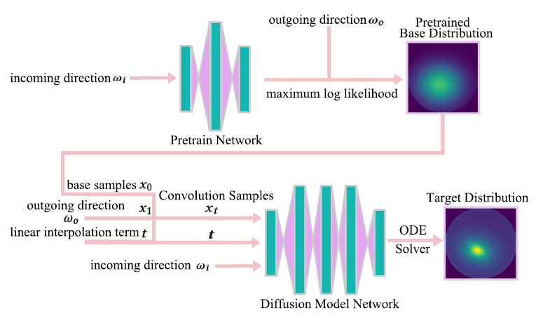
Architecture and training
- 初始分布需要方便采样和 pdf 计算
- 简单的标准高斯效果不好(太简单不够近似复杂 BSDF)
- Pretrain Network:parametric base distribution
- 例如高斯基函数,就是预测其均值和方差
- 训练:maximizing the log likelihood
- diffusion model \(D_{\theta}\) 近似
\(F\)
- 其解为:\(F(x_t,t)=\mathbb{E}\left[x_1-x_0\mid
x_t,t\right]\)
- 期望求解可以通过生成大量样本实现
- \(x_0\sim p_0\):Pretrain Network 获取的初始分布
- \(\omega_o\sim p\left(\omega_o\mid\omega_i\right)\):BSDF
- \(t\sim U(0,1)\):均匀分布
- \(x_t=tx_1+(1-t)x_0\):插值
- \(x_1=\omega_o\)
- 期望求解可以通过生成大量样本实现
- 其解为:\(F(x_t,t)=\mathbb{E}\left[x_1-x_0\mid
x_t,t\right]\)
- 训练过程:参考
- 【SIGC-2023】Iterative 𝛼-(de) blending: A minimalist deterministic diffusion model
- TODO
- 训练 loss
\[ \text{loss}=\left\|D_\theta(x_t,t,\omega_i)-(x_1-x_0)\right\|^2 \]
Training data generation
- 之前的方式【SIGC-2023】
- 先随机采样若干 \(\omega_i\),然后每个 training batch genuine
BSDF 采样 \(\omega_o\)
- 灵活,但是很慢(requires building a high-resolution histogram and perform inverse CDF sampling each time)
- 先随机采样若干 \(\omega_i\),然后每个 training batch genuine
BSDF 采样 \(\omega_o\)
- 同时我们需要训练多个网络,希望复用样本
- MCMC sampler
- 快速采样
- 使用 MCMC 预先生成样本对
- 我们使用 4D 联合分布进行采样:\(p(\omega_o,\omega_i)=p\left(\omega_o\mid\omega_i\right)p(\omega_i)\)
- 认为 BSDF \(f(\omega_o,\omega_i)\propto p(\omega_o,\omega_i)\) 是没有归一化的联合分布
- \(p(\omega_i)\) 为均匀分布
- 预先生成样本对,然后在训练的时候直接选择其中的样本对即可
- We replace the previous complex process of building histograms and inverse CDF sampling with an offline MCMC sampling
- 训练的时候,只需要生成一个随机数,预先生成的样本可以复用
Sampling
- 训练好了 \(D_{\theta}\)
- 输入 \(\omega_i\)
- pretrain network 输出初始分布系数,得到初始分布,采样生成样本 \(x_0\)
- 欧拉积分求解 ODE
- 固定步长:\(\Delta_t=1/N\)
- \(\hat{x}_{t+1/N}=\hat{x}_t+D_\theta(\hat{x}_t,t,\omega_i)/N\),\(t\in\{0,\cdots,N-1\}/N\)
- \(\omega_o=\hat{x}_{t+1}\)
- 输出的结果 \(\omega_o\) 就符合分布 \(p(\omega_o\mid\omega_i)\)
PDF evaluation
- 这是为了支持 MIS
- 每一步分布变换都是可逆的,Jacobian 可以通过自动微分得到
- 逆向 \(t=1\to0\) 即可将求 \(p(\omega_o\mid x_1)\) 转化为求 \(p(\omega_o\mid x_0)\)
- \(p(\omega_o\mid x_0)\) 能直接算出来
- 具体见补充材料(TODO)
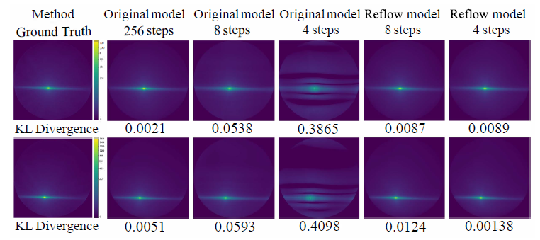
Fast and Accurate Reflow
- Reflow 论文:【ICLR-2023】
- Flow Straight and Fast: Learning to Generate and Transfer Data with Rectified Flow
- 将求解 ODE 的 Euler step 降低到个位数
- 在训练好的 diffusion model 上进行
- 需要 hundreds or thousands of Euler steps/network evaluations to ensure near-convergence
- 我们使用 tinycudann 加速
- float16 精度足够,主要就是加法,只用于生成样本,不用于 pdf 计算
- 于是现在有两个 diffusion models(这里 MCMC
的样本复用就用上了)(不太明白具体流程)
- a small network for the base weights used
for further training
- 作用:uses samples generated from large network for the Reflow process
- a large network to better capture the
distribution
- 作用:network inference, generating ODE value predictions for online sampling
- a small network for the base weights used
for further training
- Reflow 前后效果:Metal-Paper-Copper 材质
BRDF on Projected Hemisphere
- 不考虑透射,只考虑半球空间(unit hemisphere) \(\mathcal{H}\),目标是近似于 \(\text{BRDF}\times\cos\)
- 方便采样,将 \(\omega\in\mathcal{H}\) 转化为 unit disk
\(\omega_{\perp}\in\mathcal{H}_{\perp}\)
- 乘个 Jacobian
- 初始分布 \(p_0\):2D Gaussian
- 对于大部分 diffuse and (not extremely) specular materials,效果不错
- 问题:边界不连续
- 在 disk 空间中,grazing angle
的能量分布更加不均衡(看下图右侧标注),这种畸形的分布很难近似
- 接近 grazing angle 的时候很大,但是(过一点)垂直法线的时候为 0
- 在 disk 空间中,grazing angle
的能量分布更加不均衡(看下图右侧标注),这种畸形的分布很难近似
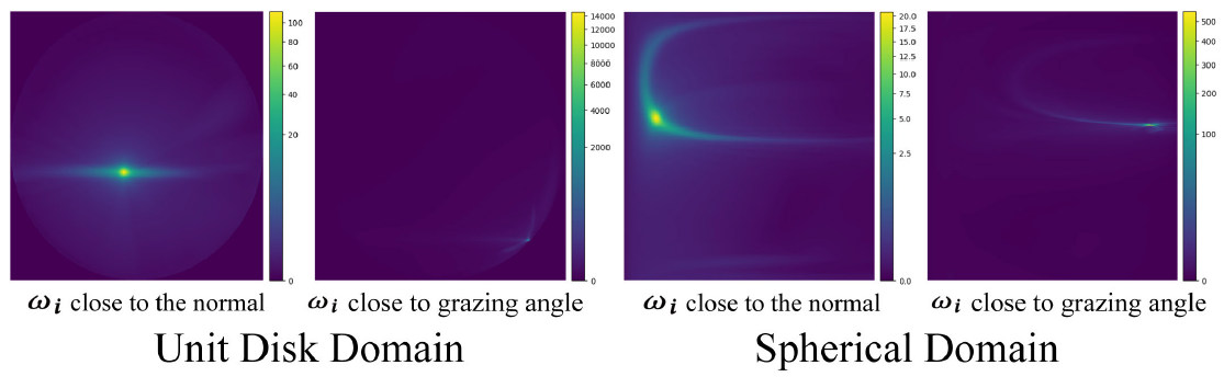
BSDF on Spherical Domain
- 能够解决 grazing angle 问题;能够扩展到透射
- 立体角:\(\mathrm{d}\omega=|\sin\theta|\;\mathrm{d}\theta \mathrm{d}\phi,\theta \in [0,\pi],\phi \in [-\pi,\pi]\)
- 在 \(\mathrm{d}\theta
\mathrm{d}\phi\) 的背景下,重要性采样变成(MC采样 \(\theta,\phi\))
- 满足基本条件:\(\theta=0,\pi/2(,\pi)\),值为 0
- 同时这样的变换让 grazing angle 附近的极大值消失了(被 \(\sin\theta\) 抵消了)(看上图右侧标注)
\[ p(\omega_0\mid\omega_i)\propto f(\omega_0,\omega_i)\cdot\left|\cos\theta\right|\cdot\left|\sin\theta\right| \]
- \(\phi\)
周期性,特殊处理,连接两个顶点 \(-\pi,\pi\)
- 映射到单位圆,使其连续
- 假设 \(p(\phi)\) 为边缘分布,条件
- \(p(\phi)=p(\phi+2\pi)\)
- \(\int_{-\pi}^{\pi}p(\phi)\;\mathrm{d}\phi=1\)
- CDF:\(c(z)=\int_{-\pi}^{z}p(\phi)\;\mathrm{d}\phi\),\(z=(z\mod2\pi)-\pi\)
- pdf、CDF 形式在 \([-\pi,\pi]\)
上不变,因此期望仍然成立
- \(x_0\) 来自初始分布
\[ \frac{dx_t}{dt}=\mathbb{E}\left[x_1-x_0\mid x_t,t\right] \]
\[ x_t=(1-t)x_0+\phi \]
- 距离测度:\(d=(x_1-x_0)\)
- geodesic distance on the unit circle
流程
- \(\theta,\phi\) 分开
- 初始分布使用两个独立的分布
- \(\theta\):使用 Gaussian
- \(\phi\):von Mises
distribution(circular normal distribution,循环正态分布):\(f(x|\mu,\kappa)=\dfrac{\exp(\kappa\cos(x-\mu))}{2\pi
I_0(\kappa)}\)
- 满足周期性
- \(\kappa\):类似方差,\([0,+\infty)\)
- diffusion model 输入
- \(\theta\)
- \(\phi\):保证其处于 unit 1-sphere,输入编码 \(\phi_{\text{input}}=(\sin\phi,\cos\phi)\)
- 一点疑问:完全把 \(\theta,\phi\) 分开了吗
Results
- 实现
- pytorch + mitsuba3
- real-time megakernel path tracer + vulkan
- 训练:pytorch + tinycudann(reflow)
- 训练过程和 BSDF 表达形式无关:只需要 \(\omega_i,\omega_o,f(\omega_i,\omega_o)\) 即可
Architecture details
- \(\omega_i\) 作为条件向量
- pretrian network:1 层 16 神经元 MLP
- diffusion model:sphere 更难学
- disk:3 层 32 神经元 MLP
- sphere:4 层 32 神经元 MLP
Baselines
- NBRDF【2021-CGF】:parametric Blinn-Phong model, isotropic(各向同性)
- NeuSample【2023-SIG】
- a Lambertian lobe and Gaussian mixtures
- Normalizing Flows
- sampling procedure provided by the RGL dataset【2018-SIG】
Materials for BSDF sampling
- RGL dataset
- complex, real-world BRDFs
- 包含 grazing angle 的材质
- BSDFs
- rough dielectric
- Disney BSDFs
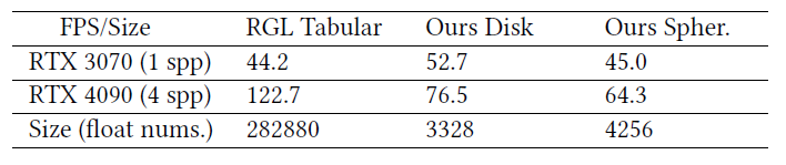
Time statistics
- a single RTX 4090 GPU
- 时间开销
- diffusion step=4
- 时间包括生成样本的计算 pdf
- 1spp,1024x1024
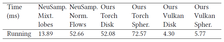
- 1spp CPU 是瓶颈,4090 L2 cache 大(72MB vs 4MB)
- 训练时间:per material averaged
- 3 hours for disk domain
- 3.5 hours for spherical domain
Better expressiveness and robustness
- 和 NeuralSample 相比,效果更好
- 能够更好处理 specular and anisotropic materials
Better compression
- 最后一行是大小,我们压缩得也很好
Spherical vs. Disk
- grazing angle 上,sphere 的 fireflier 更少
- 复杂分布,disk 更好
- disk
- 除了边界之后,都比较容易学习
- 大部分 BRDF 的能量都集中在 \(\omega_o\) 附近,让后在其周围比较均匀的分布;在 disk 域上分布更平均
Conclusion And Future Work
- future
- Better base distribution:sphere 的 von Mises distribution 存在数值问题
- Perfect transmissive materials:过大的数值引起不稳定
- Extension to SVBRDF
- Other applications:diffusion model 可以用在其他应用
- path guiding, complex luminaire sampling, and portal sampling
副录
- 推导 1
- \(x_0,x_1,t\) 独立
- \(\int f(x)\delta(x)\;\mathrm{d}x=f(0)\)
- 后面的看不懂了