(论文)[2024-EGSR] Residual path integrals for re-rendering

Posted on 2024-08-13 Edited on 2024-09-09 In CG.Paper Views:

任务是当场景中有物体发生微小变化的时候，如何从已经渲染的图像获得变化后的图像；文章提出了计算 residual integral 的方法，重要性采样变化的路径空间用于高效计算，同时提出 path mapping 充分利用前后两帧之间的相关性。

Residual path integrals for re-rendering

Bing Xu、Tzu-Mao Li、Iliyan Georgiev、Trevor Hedstrom、Ravi Ramamoorthi
项目主页
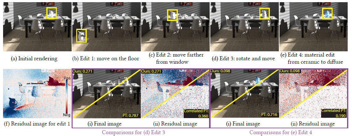
任务：移动场景中的物体，或者修改材质，更快的渲染得到修改后的图片
teaser 如下，同时间比较

Introduction

residual path integral
- 前一帧正确渲染，只渲染两帧之间的不同之处
贡献
- 将经典的 path integral 扩展到 residual path integral
- 在 residual path integral 中对 non-zero 贡献的路径进行重要性采样
- path mappings：新老路径之间的双射

Temporal reprojection
Spatio-directional caching, path guiding, and resampling
Gradient-domain rendering
Incremental radiosity
Dynamic photon mapping and virtual point lights
Scene editing and re-rendering
Portal sampling
- sampling sparse path space (e.g., lights that go through a pinhole of a scene)

Residual path integral

Primal path integral

视子路出发，初始点 \(x_0\)，BDPT 的范式（面积采样）

\[ I=\int_{\Omega}f(\boldsymbol{p})\;\mathrm{d}\mu(\boldsymbol{p}) \]

residual path integral

输入
- 前一帧的渲染结果 \(I_1\)
- 前一帧的当前帧的几何、材质配置
  - 只有微小差别，只有很小部分在变化
计算 residual：\(I_2-I_1\)

\[ I_2-I_1=\int_{\Omega_2}f(\boldsymbol{p})d\mu(\boldsymbol{p})-\int_{\Omega_1}f(\boldsymbol{q})d\mu(\boldsymbol{q}) \]

找到映射：\(\mathrm{q}=T(\mathrm{p})\)，重新参数化
- 简写：\(\Omega=\Omega_2\)
- \(f_1,f_2\)：因为路径贡献必须在对应帧的配置下计算

\[ \begin{aligned} I_{2}-I_{1}& =\int_{\Omega}\left(f_{2}(\boldsymbol{p})-f_{1}(T(\boldsymbol{p}))\left\vert T'(\boldsymbol{p})\right\vert\right) d\mu(\boldsymbol{p}) \\ &=\int_{\Omega}f_{\mathrm{d}}(\boldsymbol{p}) d\mu(\boldsymbol{p}) \end{aligned} \]

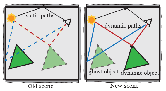
示意图
- ghost object（上一帧位置）
- dynamic object（现在位置）
- 对应修改材质，则重合

Characterizing dynamic paths

dynamic path：在当前帧下，满足下面两个条件之一，示意图
- 有顶点落在 dynamic object 上（at least one dynamic vertex）
- 有边经过 ghost object（at least one dynamic edge）
反之为 static path

Dynamic path space

small changes => 大部分是 static path => 对 residual 没有贡献
\(\Omega = \mathcal{D}\cup\mathcal{S}\)
- \(\mathcal{D}\)：dynamic path space
- \(\mathcal{S}\)：zero-contribution static path space
目的：高效采样空间 \(\mathcal{D}\)

Sampling the dynamic path space

采样从 ghost/dynamic object 出发
- 采样点 \(x_{D}/x_{G}=y_0=z_0\)
- 生成两条子路径 \(y_0\cdots y_{s-1},z_0\cdots z_{t-1}\)
  - 如果子路径只有一个点，则称为 \(x_{L}/x_{E}\)
光源：NEE，相机：light tracing（和 NEE 类似连相机？）
分类

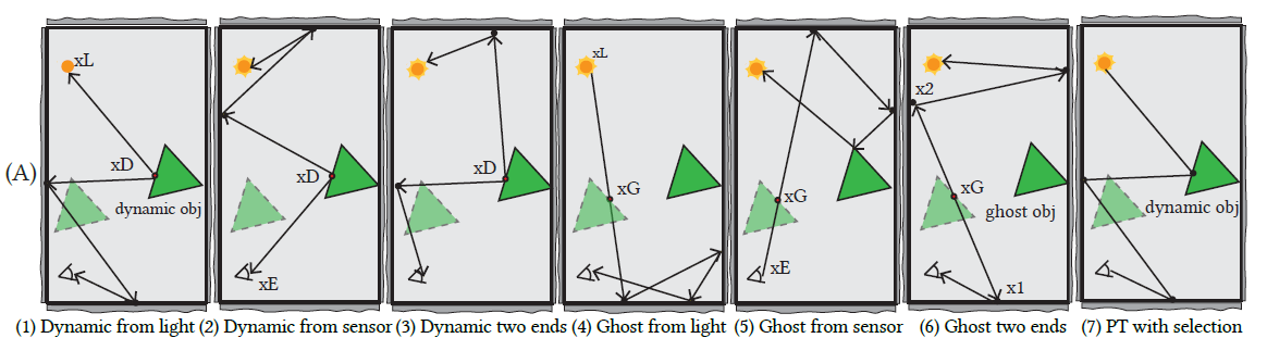
Sampling dynamic vertices

（1）Dynamic from light

light subpath 只有一个点 \(x_{L}\)
BSDF 采样 light subpath

（2）Dynamic from sensor

eye subpath 只有一个点 \(x_{E}\)，和 (1）对称
(1） (2）在直接光照下等价，3 个顶点，此时只通过 (1）处理

（3）Dynamic two ends

光源方向：法向半球采样
相机方向：BSDF 采样

Sampling dynamic edges

先在 ghost object 表面采样一个点（按面积采样）

（4）Ghost from light

面积采样得到 \(x_{G}\)（最终是不作为路径节点的）
采样光源 \(x_{L}\)
\(\overrightarrow{x_{L}x_{G}}\) 作为方向，求交得到 \(z_1\)
pdf 计算

\[ p(\bar{x})=p(x_{L})\overrightarrow{p_1}(\bar{z})\prod_{i=2}^{t-1}\overrightarrow{p_i}(\bar{z}) \]

\(p_1\)：面积转立体角转面积（这下面其实省略了微分部分 \(\mathrm{d}\)）
- 利用立体角作为中间量建立联系

\[ \overrightarrow{p_1}(\bar{z})=p(x_G)\frac{\Vert x_G-x_L\Vert^2}{\left|n_{x_G}\cdot\overrightarrow{x_Gx_1}\right|}\cdot\frac{\left\vert n_{x_1}\cdot\overleftarrow{x_Gx_1}\right\vert}{\parallel x_1-x_L\parallel^2} \]

（5）Ghost from sensor

采样相机 \(x_{E}\)，和（4）对称

（6）Ghost two ends

采样 \(x_{G}\)
均匀采样一个方向 \(p_{dir}\)，由这个方向，自然的形成点 \(x_1,x_2\)（如图）
然后向两端 BSDF 采样延伸（+NEE）
pdf 计算

\[ p(\bar{x})=\prod_{i=1}^{t-1}\overrightarrow{p_{i}}(\bar{z})\prod_{i=1}^{s-1}\overrightarrow{p_{i}}(\bar{y}) \]

\[ \begin{aligned} \overrightarrow{p_{1}}(\bar{z})\overrightarrow{p_{1}}(\bar{y}) &=p(x_{G})\cdot g_{G,x1,x2}\\ &=p(x_{G})\cdot \frac{\left\vert\cos(N_{x_1},\overleftarrow{x_1x_2})\right\vert\cdot\left\vert\cos(N_{x_2},\overleftarrow{x_1x_2})\right\vert}{\left\vert\cos(N_{x_G},\overleftarrow{x_1x_2})\right\vert}\cdot\frac{p_{\mathrm{dir}}}{\Vert x_1-x_2\Vert^2}\\ \end{aligned} \]

具体推导有两步
立体角转换为面积

\[ p_{\mathrm{dir}}=\frac{\Vert x_1-x_G\Vert^2}{\vert\cos(N_{x_2},\overleftarrow{x_1x_2})\vert}\cdot \overrightarrow{p_{1}}(\bar{y}) \]

面积转换为另一个面积，上面的（4）是一样的

\[ \overrightarrow{p_1}(\bar{z})=p(x_G)\frac{\Vert x_G-x_1\Vert^2}{\left|n_{x_G}\cdot\overrightarrow{x_Gx_1}\right|}\cdot\frac{\left\vert n_{x_1}\cdot\overleftarrow{x_Gx_1}\right\vert}{\parallel x_2-x_1\parallel^2} \]

两个式子，计算下 \(\overrightarrow{p_{1}}(\bar{z})\overrightarrow{p_{1}}(\bar{y})\) 就得到结果了

讨论

采样技术的好坏，取决于场景
如果 ghost/dynamic objects 容易连接到光源和相机，那么（3）（6）用处不大，反之效果好
如何实现整条光路的映射，看最后章节

Technique combination

MIS
例如如下情况，有 5 种采样方式
- ghost hit 作为起点（4），dynamic hit 作为起点（1）

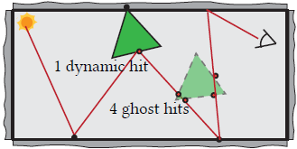
\(N_k\) 长的路径，和 dynamic object 有 \(N_D\) 个交点，和 ghost object 有 \(N_G\) 条边相交，那么就一共有 \(N_D+N_G\) 种采样策略
- 这么说的话，应该是把（1）（2）（3）区分开了（从论文中这 3 种路径的正则表达式也可以看出）
  - 3 个节点的直接光照只会被（1）采样得到
  - （3）不包括采样相机和光源
另外加上常规的 PT，用于渲染 static path（补齐整个采样空间）
- 有些光路使用 camera tracing 更容易追到
- （7）PT with selection
MIS：平衡启发式，\(N_D+N_G+1\) 种采样技术
- \(<7\)：可能连接失败，可能 rejection
计算复杂度：\(O(N_D+N_G)\)
- 在每一个点上保存累乘的 forward/backward pdf，计算的使用总的除以记录的
  - 和 BDPT 实现类似（mitsuba）
- \(O((N_D+N_G)\times N_k)\) 降至 \(O(N_D+N_G)\)

Path mapping

思路，转换为每一个节点的变换
- sensor -> emitter

\[ T(\boldsymbol{p})=T(x_0x_1\ldots x_{k-2}x_{k-1})=t(x_0)t(x_1)\ldots t(x_{k-2})t(x_{k-1}) \]

示意图

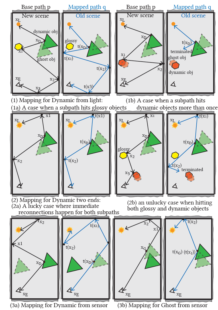
有 5 种基本变换形式 \(t\)，对应 Jacobians \(\vert{t'}\vert\)

object movement

Transform with object movement
dynamic/ghost obejct 上的刚性变换
\(t(x_i)=T_{obj}(x_i)\quad\mathrm{if}\quad x_i\in\{x_D,x_G\}\)
For rigid motions of articulated bodies, \(\vert{t'}\vert=1\)
如图（1b）所示，如果 base path 和 dynamic obejct 有多个交点，则拒绝映射（如何处理？）
- 可能会引发很大的区别

same vertex

Keep vertex the same
static object 上的顶点不变
\(t\left(x_{i}\right)=x_{i}\quad\mathrm{if}\quad x_{i}\in\{\mathbf{x}_{S}\}\)
\(\vert t'\vert=1\quad\mathrm{if}\quad t\left(x_{i-1}\right)=x_{i-1}\)
这样的操作允许 path re-connection（前一个点 \(x_{i-1}\) 可以和当前点 \(x_i\) 连接）
此时，如果 \(x_{i-1}\) 被映射到了另外的点，\(\vert t'\vert\) 不再是 1

\[ \mid t'\mid=\frac{\cos\left(t\left(x_{i-1}\right)\leftarrow x_i\right)}{\cos\left(x_{i-1}\leftarrow x_i\right)}\cdot\frac{\Vert x_{i-1}-x_i\Vert^2}{\Vert t\left(x_{i-1}\right)-x_i\Vert^2}. \]

一个 path 避免多次连接（可能导致很大的 Jacobian）
- Jacobian 的累乘
连接条件：参考 ResTIR
- \(x_i\) 不是 dynamic vertex
- roughness threshold：\(\min\left(\alpha(x_{i-1}),\alpha(t(x_{i-1})),\alpha(x_{i})\right)\geq\alpha_{min}\)
- distance threshold：\(\min\left(\|t(x_{i-1})-x_{i}\|,\|x_{i-1}-x_{i}\|\right)\geq d_{min}\)

random replay

Random-seed replay
使用同样的随机数生成 ray \(\overrightarrow{x_{i-1}x_{i}},\overrightarrow{t(x_{i-1})t(x_{i})}\)

dynamic/ghost pair

Mapping between the dynamic and ghost pair
直接映射到对应点，然后继续光追
- 上图的 3a、3b

Path rejection

Path rejection
当 path mapping 失败或者主动停止时，使用这个方案
主动停止条件
- mapped path 重连的时候被遮挡（或被 dynamic obejct 遮挡）
- Jacobian 超过阈值（导致 fireflier），设置为 10
- base path 多次击中 dynamic object（>1）
条件1、3 发生较少，因为移动较少
- dynamic objects 占据较多时发生多
条件 2 发生更少
具体方式，无偏性的保证
- we sample from both frames and employ two-way path mapping to ensure the coverage of the entire integral domain.
- 和论文类似：Improved sampling for gradient-domain Metropolis light transport

Results and discussion

实现

渲染器：Intel Embree
AMD Ryzen 16-Core Processor
额外维护两个加速结构：dynamic/ghost obejcts
- dynamic：连接的时候可见性测试
- ghost：计算 MIS 需要
- 代价很小：只有少部分会移动
无偏测试：能收敛到 reference

Incremental re-rendering

对比算法：PT，Correlated PT
PT：只考虑移动物体对相机直接可见的场景（公平性）
- 感觉对 PT 不应该都一样吗？对 residual 难度不一样？
- 大部分测试场景都是 PT 友好的
Correlated PT：不太懂具体怎么做的
- 渲染 residual，然后累加
比较 reference、residual reference 的区别
- 等时间的 MSE 都低
dynamic object 距离光源越近，residual 越大
- 我们的方法不管距离怎么变化，收敛都很快
- 在这种情况下，直接 PT 有可能会更好
Scene Editing
- 当光源/相机移动的时候，最优的退化为 light/camera tracing
- 材质编辑则比较简单，不需要 MIS 采样那一大堆

Timings and overhead

光线从中间物体出发，cache miss 很严重
- 留到 future work：potential batching and coherency optimization
- 计算开销：10-20%
- 因此，同时间对比中，PT 有更多光线（random walk）

Ablations and analysis

只展示变化部分（\(\mathcal{D}\)）
- PT with selection：path tracing where only the paths affected by the dynamic objects are selected and contributing to the shown image
- 论文效果更好（比 PT 好）
path mapping 是否开启
- 关闭：不做 mapping，而是在两帧图像中各自采样论文中的采样策略，计算图像
- path mapping 有效
当移动的物体变多，论文方法变差
- 论文假定：变化东西很少
当物体变化的量变大，论文方法能保持一致，但是 path mapping 作用减弱

Limitations

可以和 light/camera tracing 结合
算法不适合 camera/light 移动的场景
不同的 dynamic/ghost 上的方差不同：适应性采样

结果与展望

Conclusion
- theoretical framework
future work
- better importance sampling techniques
- better path mappings
- 上面二者联合优化
- 支持 deformable movement
- 参与介质（体渲染）

整条光路的映射

base path \(\boldsymbol{p}\) from new scene \(\to\) old scene
标准 PT 可以让帧间使用相同的随机数，以增强相关性；动态场景则比较难
- 我们的方法起点在光路中间，不确定是在哪个像素，因此很难使用这个
核心思想：尽早的进行 path reconnection，原因如下
- efficiency, in terms of path reuse
- increasing correlation between the two paths
连接之前使用 Random seed replay（增强相关性）
Dynamic from sensor
- 图上的 1a 是一个例子，\(x_1\) 无法连接，因为 glossy 条件；直到 \(x_3\) 才满足连接条件
- 图上的 2 也是满足的例子
Dynamic from sensor
- 3a 中 \(t(x_D)\) 延长线的交点和 \(x_1\) 不连接，是因为 large Jacobian
- 当物体移动过大的时候，Dynamic from sensor 使用 Transform with object movement 策略，效果不好，相关性很差
- 这里使用直接延长的策略
- Ghost from sensor 也类似
Ghost from light、Ghost two ends 这两种情况
- 直接使用 independent tracing
- 使用和上面差不多的方式，相关性较差；原因是 ghost 都是空的，会打到其他物体，从而贡献给其他像素

总结

满抽象的，不太理解无偏性的保证
- 这个 mapped path 的形成方式是唯一的吗？不唯一的话需要计算 pdf 吧
- 无偏的原因？
  - 和 dynamic object 只会有一次相交，在采样前的操作的都是确定性的操作