(论文)[2020-HPG] ꟻLIP: A Difference Evaluator for Alternating Images
TLDR
- 输入为 LDR 的 RGB 图片,范围 \([0,1]\)
- color pipeline
- RGB -> \(\text{Y}_{\text{y}}\text{c}_{\text{x}}\text{c}_{\text{z}}\) -> 空域滤波(频率低通,高斯近似,逆傅里叶变换到空域加速)-> RGB -> clamp -> \(\text{L}^{\ast}\text{a}^{\ast}\text{b}^{\ast}\) -> Hunt 调整 -> 计算 metric(firefliers 的存在,需要压缩大的 error)
- feature pipeline
- edge detection:2D 高斯一阶导数
- point detection:2D 高斯二阶导数
ꟻLIP
- ꟻLIP: A Difference Evaluator for Alternating Images
- 为了方便,下文都直接用 FLIP
- Pontus Andersson, NVIDIA
- 项目主页
- 代码
Introduction
- Flipping/Alternating 两张图片,比把两张图片并排放着,更能够看出两张图片的异同
- 现在比较的方式:用户很难直观感受到区别
- 并排放图片AB
- A切换空白再切换到B
- 渲染研究者希望是:A直接切换到B(最直观)
- FLIP:希望解决上面这个问题,同时考虑 error map(误差图)的影响
- 之前的方法大多是为了解释用户对刺激的反应,而不是考虑误差图
- 对于颜色、边界的考虑借鉴了 models of the human visual system
- 基于渲染,还考虑了 point-like structures(例如 fireflies)的影响
- full-reference image difference algorithm
- 输出一张图片,表示 difference
- 收到 iCAM framework 的启发,评估包括
- contrast sensitivity functions
- feature detection models
- a perceptually uniform color space
- 试图实现和人类感知一致的 metric
- 做了用户实验
- 包括自然图片与生成图片
Goals and Limitations
- FLIP 的 error 希望正比于人眼在切换图片时的感知 error
- flipping back and forth between the images, located in the same position and without blanking in between.
- 和观察者的距离、像素分辨率相关
- 需要选择一个 color space 和距离成正比
- perceptually uniform color space
- 需要选择一个 color space 和距离成正比
- point content(fireflies)、edge content 的变化对于感知来说比较明显
- 需要特别重视
- flipping 这个操作对于渲染来说很重要,大家都是这样看 error 的
- 设计理念
- ease-of-use
- 复杂度低
- 用户指定的参数要少
- 不能处理 HDR 图片
- 无法检测视觉掩蔽现象(visual masking)
- 当一个视觉刺激(目标刺激)被另一个或多个同时呈现的视觉刺激(掩蔽刺激)所干扰时,目标刺激的感知能力降低的现象。简单来说,就是一些视觉元素会干扰我们对其他元素的识别。
- 但是我们的算法无法识别(计算机不会被干扰)
Previous Work
- 一个 Survey:Seven Challenges in Image Quality Assessment: Past, Present, and Future Research
- 分类:根据需要 reference 的程度进行划分
- full-reference algorithms(FLIP 是这种)
- reduced-reference algorithms
- no-reference algorithms
- 分类:出结果
- 输出一个值:Guetzli(2017)、PieAPP(2018-CVPR)、Multi-scale Structural Similarity(2003)
- 每个像素输出一个值(FLIP
只对比这种)
- 表示这个像素有误差可见的可能性:HDR-VDP-2(2011-SIG)、CNN-based
metric(2018-TOG)
- where the distortions are visible
- 表示这个像素误差的大小:iCAM(2004)、S-CIELAB and CIEDE2000(2003)、SSIM(2004-TIP)、deep features(2018-CVPR)
- 表示这个像素有误差可见的可能性:HDR-VDP-2(2011-SIG)、CNN-based
metric(2018-TOG)
- 对比场景:alternating images with no blank image shown between the flips
对比算法
- Symmetric mean absolute percentage error (SMAPE)
- 应用:降噪网络的训练
- SSIM
- 与:average value, the variance, and the correlation of luminances 相关
- S-CIELAB(FLIP 继承和发展了这个方法)
- 考虑了 human visual system (HVS)
- filter the images using contrast sensitivity functions
- 在 perceptually uniform color space 中计算距离
- HDR-VDP-2
- 输出 error 被发现的概率,HDR(设计应用)/LDR 都可以使用
- 网络
- 网络的中间表示能用于计算区别
- PieAPP:网络输出每张图的失真程度
- user markings:输出 visibility map
- Butteraugli:part of the Guetzli system to optimize JPEG compression
Algorithm
- FLIP 输出 error map,每个点的值正比于感知误差的大小
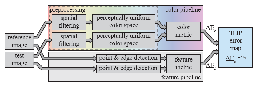
- FLIP pipeline 如下
- color pipeline
- spatial filter
- 基于 human visual system’s contrast sensitivity functions (CSFs)
- 去除在给定观察距离、给定像素分辨率下感知不到的高频信息
- 转化成:perceptually uniform color space (PUCS) \(\text{L}^{\ast}\text{a}^{\ast}\text{b}^{\ast}\)
- one achromatic(明度)and two chromatic components(颜色相关)
- 简单,但是有缺陷
- 不能处理 Hunt effect(随着亮度的增加,人们对颜色的感知也会变得更加鲜艳)
- 为了处理 Hunt effect,我们做简单调整
- 计算 difference,映射到 \([0,1]\)
- spatial filter
- feature pipeline
- color pipeline
Color Pipeline
- 输入为 sRGB(\(\{R_s,G_s,B_s\}\)),处理完之后要考虑 Hunt 效应(低亮度的 chromatic errors 要变小)
Spatial Filtering
Step 1
- 先线性化成 \(\{R',G',B'\}\)
- standard linearization formula
- 代码里是这么写的,3 通道分别计算
1 | // cpp/FLIP.h |
- spatial filtering 在补色空间中做
- CSFs 中:1 achromatic channel, 1 red-green channel, and 1 blue-yellow channel
- S-CIELAB research 中使用的会带来 undesirable color shifts
- 我们选择 \(\text{Y}_{\text{y}}\text{c}_{\text{x}}\text{c}_{\text{z}}\)
空间(\(\text{L}^{\ast}\text{a}^{\ast}\text{b}^{\ast}\)
的线性版本)
- \(\text{Y}_{\text{y}}\):achromatic channel
- \(\text{c}_{\text{x}}\):red-green channel
- \(\text{c}_{\text{z}}\):blue-yellow channel
- 转换
1 | pImage[i] = color3::XYZToYCxCz(color3::LinearRGBToXYZ(pImage[i])); |
具体转换逻辑如下,点击展开
1 | HOST_DEVICE_FOR_CUDA static inline color3 LinearRGBToXYZ(color3 RGB) { |
- 现在得到了 \(\{S_{\text{Y}_{\text{y}}},S_{\text{c}_{\text{x}}},S_{\text{c}_{\text{z}}}\}\)
Step 2
- CSFs 对于敏感度的定义:cycles per degree of visual angle 的函数
- 我们这里进行转化,one cycle corresponds to two pixels
- 与观察距离和像素分辨率相关,计算 PPD(pixels per degree)\(p\)
- 观察距离 \(d\) 米
- 显示屏大小(单位米):\(W_{\text{m}}\times H_{\text{m}}\)
- 分辨率:\(W_{\text{p}}\times H_{\text{p}}\)
\[ p=d\dfrac{W_{\text{p}}}{W_{\text{m}}}\dfrac{\pi}{180} \]
Step 3
- 频域滤波:选择滤波器,频率滤波转换为空域滤波,\(3\sigma\) 确定空域的范围
- 我们是基于 1988 年的 CSFs,但是这些 CSFs 不是度量 \(\text{Y}_{\text{y}}\text{c}_{\text{x}}\text{c}_{\text{z}}\)
空间的
- 但是这个带来的 inaccuracy 是微不足道的
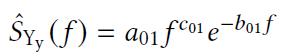
- CSFs:频域
- achromatic CSF:带通滤波器(bind-pass filter)
- chromatic CSF:低通滤波器(low-pass filter)
- 我们需要保留直流分量(DC),因此都修改为低通
- 直流分量表示平均值(不变的)
- low-pass filter 如下
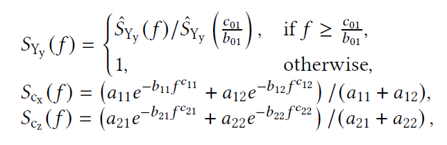
- GPU 快速 filter,将其转化为 Gaussians 的和
- 直接使用上面的低通会导致振铃效应(ringing artifacts)
- 每个通道,我们使用 1-2 个 zero-centered Gaussian 代替
- 频域高斯
\[ G(f)=ae^{-bf^2} \]
- 转化为空域(逆傅里叶变换):\(\sigma=\sqrt{\dfrac{b}{2{\pi}^2}}\)
\[ g(x)=a\sqrt{\dfrac{\pi}{b}}\exp(-\frac{\pi^2}{b}x^2) \]
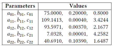
- 使用 Matlab
找到最优近似:近似的时候是近似频域得到最优的 \(b(,a)\)
- filter 之后有归一化,因此如果只有一个 Gaussian 的话,倍数系数不用管
- 两组表示两个
| 参数 | 值 |
|---|---|
| \(b_{\text{Y}_{\text{y}}}\) | 0.0047 |
| \(b_{\text{c}_{\text{x}}}\) | 0.0053 |
| \(a_{\text{c}_{\text{x}}},b_{\text{c}_{\text{x}}}\)(2 组) | (34.1,0.04), (13.5,0.025) |
- 频域区间:\(\left[-\dfrac{p}{2},\dfrac{p}{2}\right]\),\(p\) 为采样频率
- S-CIELAB and CIEDE2000 工作
- 转换为空域:\(\Delta=\dfrac{1}{F_s}=\dfrac{1}{p}\)
- \(\Delta\):刚好对应频率中最近的两个采样点在空域中的距离
- 单个高斯模型,\(3\sigma\) 保留了 99.7% 的能量
- 因为我们使用的高斯都是 zero-centered,使用最大的 \(3\sigma\) 就能保证所有高斯都保留 \(\ge\) 99.7% 的能量
- 这里直接考虑保留空域中高斯的 \(3\sigma\)(神奇,我还以为会考虑频域,转化到空域)
- \(b_{\max}=0.04\)
\[ \begin{aligned} r_{\max} &=\left\lceil{\sqrt{\dfrac{3\sigma_{\text{space}\max}}{\Delta}}}\right\rceil\\ &=\left\lceil{\sqrt{3p\cdot\dfrac{b_{\max}}{2{\pi}^2}}}\right\rceil\\ \end{aligned} \]
- 1D filter 的范围
\[ 0,\pm\Delta,\pm2\Delta,\cdots,\pm r\Delta \]
- 2D filter 的范围
\[ \begin{array}{c} \text{evaluate}:d(x,y)=\Delta\sqrt{x^2+y^2}\\ (x,y),x,y\in\{0,\pm1,\pm2,\cdots,\pm r\}\\ \end{array} \]
- 权重归一化
- 现在得到了 filtered colord \(\left\{\widetilde{\text{Y}}_{\text{y}},\widetilde{\text{c}}_{\text{x}},\widetilde{\text{c}}_{\text{z}}\right\}\)
- 需要转换到 RGB 空间,然后 clamp 到 \([0,1]^3\) 之间
- 不然 filter 之后可能超出 RGB 范围
Perceptually Uniform Color Space
- 这个空间中的距离和感知距离成正比
- clamp 之后的 RGB 转化到 \(\text{L}^{\ast}\text{a}^{\ast}\text{b}^{\ast}\) 空间,得到 \(\left\{\widetilde{L^{\ast}},\widetilde{a^{\ast}},\widetilde{b^{\ast}}\right\}\)
1 | // Move from linear RGB to CIELab. |
LinearRGBToXYZ上面有了
具体转换逻辑如下,点击展开
1 | HOST_DEVICE_FOR_CUDA static inline color3 XYZToCIELab(color3 XYZ, const color3 invReferenceIlluminant = INV_DEFAULT_ILLUMINANT) { |
- 考虑 Hunt 效应:除了亮度都一样
| 亮度低,对比弱 | 亮度高,对比强 |
|---|---|
  |
  |
转换为 \(\left\{\widetilde{L_{\text{h}}^{\ast}},\widetilde{a_{\text{h}}^{\ast}},\widetilde{b_{\text{h}}^{\ast}}\right\}\)
\(L\) 本身范围就是 [0, 100],\(a,b\) 没有限制
直观上理解:给 \(a,b\) 的差距乘上 \(L\) 作为系数
![]()
![]()
Color Metric
- 之前的 metric 只在 distance 比较小的时候有用
- 渲染的 distance 可能很大:fireflies
- HyAB:a metric designed to handle larger color distances
- HyAB distance, \(\Delta\text{E}_{\text{HyAB}}\)
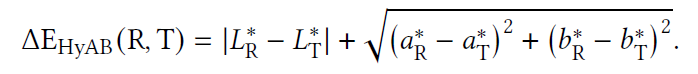
- 最大为 \(308\)
- 输入 RGB 为(\(\{0,0,1\},\{0,1,0\}\))
- 全黑白是 \(100\)
- reduce the gap between large differences in
luminance versus large differences in
chrominance
- 高端(接近 1 部分)压缩
- 进行一个映射:\(q_c=0.7\)
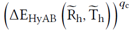
- 映射之后
- 此时上面最大值为:203(Hunt adjusted 之后变了,但还是最大值)
- \(q_c\) 映射之后:41
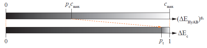
- 之后再归一化到 \([0,1]\)
- 归一化的时候,进一步对 big value 进行压缩
- 给两个超参:\(p_c=0.4, p_t=0.95\)
- 映射:输入为 \(\Delta\text{E}_{\text{HyAB}}\)
- \([0,p_cc_{\max})\to[0,p_t)\):线性映射
- \([p_cc_{\max},c_{\max}]\to[p_t,1]\):用上面的压缩
- 映射:输入为 \(\Delta\text{E}_{\text{HyAB}}\)
- 给两个超参:\(p_c=0.4, p_t=0.95\)
Feature Pipeline
- 之前的工作能比较好检测 edge,但是对 point 不太行
- 两张图都过一遍,对比响应不同的地方
Feature Detection
- 转换到 \(\text{Y}_{\text{y}}\text{c}_{\text{x}}\text{c}_{\text{z}}\)
空间,然后在 \(\text{Y}_{\text{y}}\) 做
feature detection
- 高频空间信息基本都在这个通道上
- 归一化到 \([0,1]\)
- 输出值都在 \([0,1]\) 之间
- kernel 卷积,权重和都为 1/-1
- ppd(\(p\))相关(pixel per angle)
- edge 检测:2D 对称高斯的一阶微分
- 人眼对边缘的响应:\(\omega=0.082 \deg\)
- 我们使用的 filter 的标准差:\(\sigma(w,p)=\dfrac{1}{2}wp\)
- filter 半径为 \(3\sigma\)
- \(\lceil3\sigma(\omega, p)\rceil\) pixels
- 实现上,\(x,y\) 方向各来一遍,得到的图片记作 \(\Vert\nabla \mathrm{I}\Vert\),每个像素对应的值称为 edge feature value
- point 检测:2D 对称高斯的一阶微分
- 参数和实现都类似
- 得到的图片记作 \(\Vert\nabla \mathrm{I}^2\Vert\),每个像素对应的值称为 point feature value
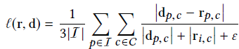
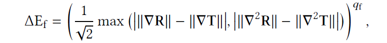
Feature Metric
- edge/point 不太会出现在同一个像素里
- \(q_{\text{f}}=0.5\)
- \(/\sqrt{2}\):让结果在 \([0,1]\) 之间,为啥?
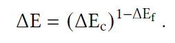
Final Difference Map
- 都是 \([0,1]\)
Pooling
- 降分辨率,特殊的变成一个值
- 信息不可逆的丢失
- 压缩数据
histogram
- histogram:\(x\to n(x)\)
- weighted histogram:\(n\to x\cdot n(x)\)
- spp 越高,error 越集中在小的部分,但是高 error
的数量也在增加(firefly 的概率在增加)
- firefly 的问题可能导致 spp 增加时,error 有所增加
- 进一步压缩
- weighted median and the arithmetic mean
- mean:容易求导,可以用于 NN
- 25% and 75% weighted percentiles (first and third weighted quartiles):分位数
- the minimum value, and the maximum value
- weighted median and the arithmetic mean
Evaluation
- 两个部分
- analyze the error maps
- user study
- 数据集
- 自己生成
- 前人:LocVis、the CS-IQ image data bases、\(\cdots\)
- artifacts 类型
- aliasing、Monte Carlo noise、color shifts
- 退化的自然图片:compression、dither(抖动)、blur、contrast changes
- 对比 metric:为了展示,都调整输出到 \([0,1]\)
- HDR-VDP-2、LPIPS、the CNN visibility metric(CNN, for
short)、Butteraugli
- 输出的 \([0,1]\),error 小到大,修改他们的 color 映射到我们这个
- SMAPE:一般用于 HDR
- Euclidean RGB distance
- 可能的最大值认为是 RGB cube,归一化
- S-CIELAB
- 最大值为 259(blue、green)
- SSIM:\([-1,1]\)
- no error:1,max error:0
- negative values can arise due to the correlation factor
- \(s'=1-s\)
- PieAPP:\((-\infty,\infty)\)
- no error:0,max error:\(\pm\infty\)
- \(a'=\left\vert{2-\dfrac{1}{1+e^a}}\right\vert\)
- HDR-VDP-2、LPIPS、the CNN visibility metric(CNN, for
short)、Butteraugli
- 项目主页上有展示
Analysis
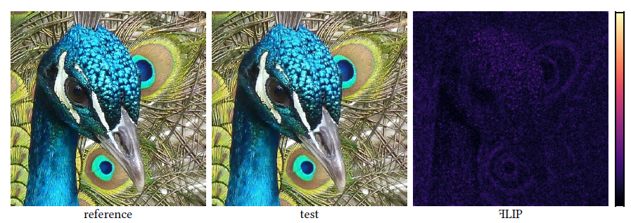
Figure 9
- 每一个方法和 FLIP 比一张图
- CNN、LPIPS、PieAPP
- 定位不准(网络方法的通病)(localization)
- 会将 error 部分的周围也当作 error(扩散)
- HDR-VDP-2
- ringing artifacts
- 但是说实话这里 diffuse 的那种噪声 FLIP 显示的不好
- Butteraugli
- 偶尔会对不明显的差异反应过度
- localization 问题
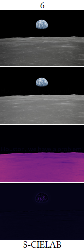
- S-CIELAB
- band-pass filter 的问题,会导致全局的 blur
- filter 之后平均了整体的灰度,导致结果上相似,error 不见了
- band-pass filter 的问题,会导致全局的 blur
- SSIM
- 没有考虑 pdd,导致将很多观察不到的误差都展示出来了
- 有一些不可解释的结果值
- SMAPE
- 因为除了像素真值(relative error),导致暗处误差放大,但实际上这些观察不到
- FLIP 通过 Hunt-adjustment 克服了这一点
Figure 10
- MCPT 不同 spp 结果,所有方法比 error
- 一致性:spp 增加,error 变小(特殊:firefly 增多)
- FLIP
处理不了的问题:masking(有大的不同,但是因为其他原因我们观察不到)
- where image differences are present, but also hard to notice due to high amounts of irregularities or contrast shifts
- FLIP 会 overestimation,下图是一个示例
- 性能:180 ms
- unoptimized GPU implementation
- \(p=67\text{ PPD}\)
- 1920 × 1080
- NVIDIA RTX 2080 Ti
User Study
- ref/test flip 切换,周期为 0.5s(每秒两张图?)
- 图片顺序随机
- 不同 metric 的 error map 的顺序也是随机的
- 用户
- 打分:0-3(metric 和 error 对应的差到好)
- 关注异常
- false positives (indicating differences when there are none)
- false negatives (not indicating differences when they exist)
- 关注 magnitude and localization
- 距离满足 \(p=67\) pdd
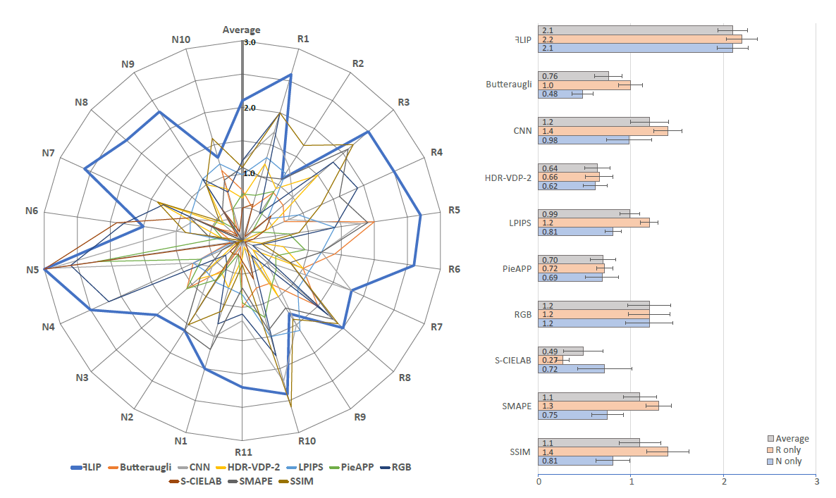
- 数据组成
- 11 组 rendered images(R)
- 10 组 natural images(N)
- 8 其他数据集
- 2 我们进行 distortion
- 用户
- mainly computer graphics experts
- 还包括 color scientists and computer vision researchers
- 结果如下:FLIP 平均分数 2.1
Discussion
- FLIP 好的原因:主要和上面的分析类似