(论文)[2024-SIG-C] N-BVH: Neural ray queries with bounding volume hierarchies
TLDR
- 任务:光追背景,输入光线,输出交点、albedo、normal
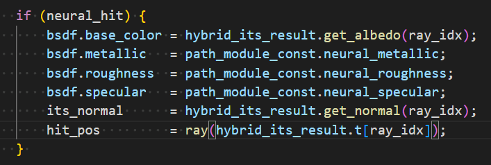
- 生成反射光线:交点+normal(+场景中写死的BSDF参数)
- 创新点:压缩场景(速度差不多、结果可接受的情况下,显存变为10%)
N-BVH
- N-BVH: Neural ray queries with bounding volume hierarchies
- Philippe Weier,DFKI,Saarland University
- 论文:作者网站
- 代码:Github
摘要
- 神经网络在压缩信号方面很有效
- 渲染中,大量存储被用于纹理和几何
- 压缩!
- 挑战:训练时间短、推理时间快的 trade off
- multi-resolution hash grid
- 使用 adaptive BVH-driven probing scheme 优化参数
- 可以将 non-neural 和 neural 的方法结合,取各自的长处
- 论文:Neural BVH or N-BVH(\(\mathcal{N}\text{-BVH}\))
- 可以实现
- accurate ray queries
- faithful approximations of visibility, depth, and appearance attributes
Introduction
- BVH:加速光线与场景求交
- 问题:内存(显存)占用过大
- Our key observation is that any neural compression
model can be optimized efficiently as long as it is trained on samples
that live close to the signal of interest.
- 神经网络总是能过拟合
- 训练:使用场景的 BVH 生成 ray queries/responses 数据对
- 几分钟
- 推理:和 BVH 类似,但是不需要 full, deep BVH traversal and hence storage
- N-BVH 可以和 standard BVH 一起使用
- N-BVH 还有一套 simple level-of-detail (LoD) scheme
- hash grid 的好处:稀疏编码
- faster and easier training
贡献
- N-BVH 的数据结构
- neural ray-intersection query mechanism
- fast training scheme driven by a coarse-to-fine tree-cut
optimization
- 哪里误差大优化哪里
- multiple adaptive neural levels of-detail
应用场景
- hybrid path tracing
- neural appearance prefiltering
Related Work
- Neural implicit representations(神经隐式表示)
- NeRF
- novel view synthesis
- 位置编码:稀疏编码、压缩编码
- NeRF 相关
- accumulating features along rays 从而减少 dense MLP queries 的负担
- tree-structured MLP(improve compression fidelity)
- further speed and accuracy can be gained with an adequate empty-space
skipping strategy
- 减少 MLP 查询、提高信号质量(采样的都是表面附近的)
- Geometric simplification(几何简化)
- Silhouette and shape-preserving decimation(often with artist supervision)
- ...
- Neural compressed geometric reconstruction(神经压缩的几何重建)
- 使用 SDF 替代 Mesh 表示
- 提出(慢、低频)
- octree feature volume:高频
- optimized space partitioning:高压缩率、准确
- 直接再三角形上做
- learning
visibility and depth for arbitrary ray queries
- ray-foot parameterization 避免相同交点的混淆(\((p,d),(p+\delta d,d)\) 结果应该相同,但是简单的编码,网络很难输出相同结果)
- 没有对几何做压缩,因此需要很大的 MLP 进行推理
- visibility:这里的可见性指的是,只学到了最外层的点吧
- Neural VDB
- 使用 SDF 替代 Mesh 表示
- Hybrid neural path tracing
- shadow ray 可见性问题:Neural Intersection Function(AMD)
- 过拟合光源和相机位置,交互性差、不能 relighting
Method Overview
- 使用神经网络替代 BVH Mesh
- infer intersection point, surface normal, and appearance.
- 基于 multi resolution hash grid
- Neural ray inference
- 存在误差
- 网络大小、输入编码都会影响网络性能
- 让样本都在表面附近 \(\to\) 高效
- 密集采样太慢了,传统 BVH 做指导(在相交的 BVH 中进行采样)
- a single global neural model 编码整个场景几何
- 最终:no geometrical primitives, no textures, and only a shallow BVH
- 压缩率高
Neural Ray Query
- 训练:几何元素+包围盒 \(\to\) 交点信息
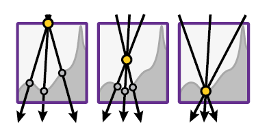
Motivation
- query 最简单的参数化:ray-box entry and exit points
- 效果差
- 这种编码和要学习的信号(交点)相关性差
- 导致 blur、loss in accuracy
- 下图以 entry point 为例
- 相同的入射点,交点相差很大(网络学习到平均信息)
- 如果 encoding point 更加接近表面,那么差距越小
- 最理想的话直接就是交点
- 效果差
Network
- Encoding, inference & training
- 我们不知道交点(正是我们想计算的)
- 输入
- 采样若干个点形成 ray-box intersection interval
- 保存到 multi-resolution grid 里面(经过 grid 之后,position 变成 feature)
- concatenate(有序的,编码了方向)
- 过小 MLP
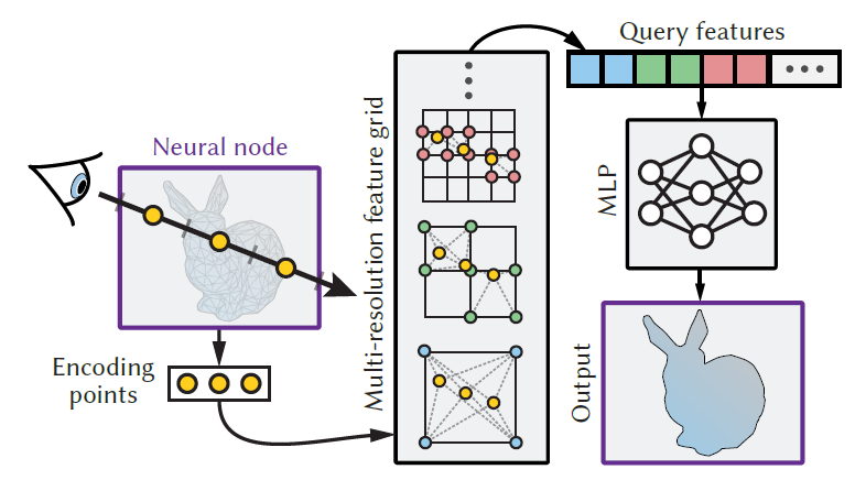
- pipeline
- 采样光线
- 均匀的场景中采样起点,50%-inflated scene bounding box(50% 膨胀的场景 AABB 包围盒)
- 均匀采样一个方向
- 输入模型
- 真实值(GT)为光线与场景求交的实际结果
- 采样光线
- loss:根据具体信号具体设计
- 优化:梯度下降
Sampling
- Sampling & reconstruction quality.
- 光线的编码:光线上的若干个点
- 采样点
- 例如:光线上采样 2 个点,则采样点位置为 25%,75%
- \(x\to\dfrac{2i+1}{2x}\),\(i=0,\cdots,x-1\)
- 例如:光线上采样 2 个点,则采样点位置为 25%,75%
- 当有一个样本点在物体表面(第一个交点)的时候,效果好
- 例子:45度倾斜的棋盘格
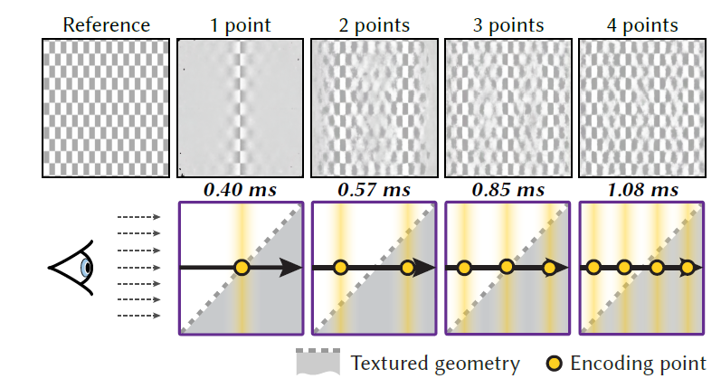
- 期望靠近表面
- naive:增加采样个数,开销增大
- N-BVH 解决了这个问题(使用 BVH 做引导)
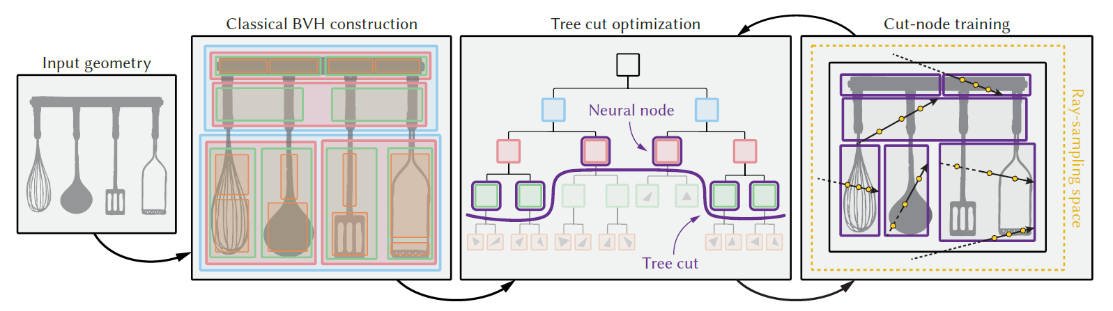
Neural BVH
- 期望光线上的采样点靠近物体表面
- 使用场景 BVH 作为引导,只需要考虑相交的 ray segment
- We split the input geometry into smaller, simpler pieces, enclosing each in a tight bounding box.(似乎作者的 BVH/三角网格 特别精细?)
- 实现了我们的目标
- front-to back ray traversal
- empty-space skipping
- probing the model closer to the geometry
- 一条光线总的查询次数(neural queries):在找到交点之前碰到的 BVH 叶子节点个数
- 一个浅层的 N-BVH 比使用单个 neural node 效果好很多,如下图
- 第一排:每一个节点的平均 training loss 可视化
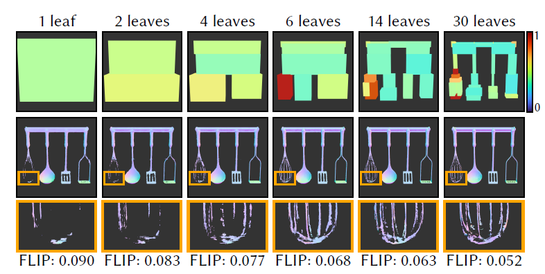
- N-BVH 的结构
- 和传统的 BVH 相比,节点数量更少(少1-2个数量级)
- Nerual Node 是空心(hollow)的,具体内容是保存在1个大的网络中
Error-driven construction
- 想要让场景的 inference error 差不多(叶子结点的 error 相同),见上面的可视化
- top-down approach
- switch between model training & node splitting
Base-BVH cut optimization
- 直接使用场景 input-geometry 的 BVH(base BVH)
- 迭代法找到 Tree-cut(含义见图)
- 每轮迭代:将 cut 移动的更深,cut 相邻的浅层节点作为 Neural
Node
- 先训练网络
- 找到最大 error 的结点,使用他们的子节点替代(将子节点作为 Neural
Node)
- 分裂几个节点(top-k),由用户指定
- 迭代次数
- 用户指定 Neural Node 的个数,当达到用户指定值的时候,停止迭代
- 随着迭代次数增加,cut 变大,Neural Node 增多
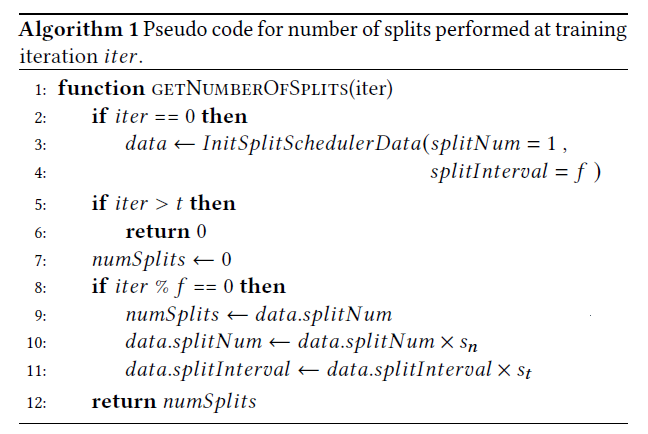
- 详细算法
- frequency \(f\):迭代多少次分裂 nodes(更新 tree cut)
- scaling factor \(s_n>1\):每次分裂数目不一样,越来越多
- scaling factor \(s_t>1\):间隔时间越来越长(tree-cut 变大了,需要更多样本训练)
- 参数:\(t=3000,s_t=2\)
| Target node count | \(f\) | \(s_n\) |
|---|---|---|
| 7 | 3000 | 2.0 |
| 155 | 300 | 2.0 |
| 1.2k | 100 | 2.0 |
| 11k | 50 | 2.3 |
| 33k | 40 | 2.5 |
| 73k | 50 | 3.2 |
| 142k | 90 | 5.0 |
Node error
Neural Node 的 error 如何评估?
\(q\cdot p\):具体的见下一个 section
- \(q\):node 的 training loss
- \(p\):random ray hit it 的概率
- 正比于 node 的表面积(因为训练的时候光线是均匀分布在场景中的)
- 实际实现的时候,我们使用击中当前 node 的光线比例进行估计
使用 \(r\) 替代
- \(r=2\log q+\log p=\log(q^2p)\)
- 直接使用 top-k 的 \(p\cdot q\) 会导致对于 large and/or high-loss nodes 的过度激进分裂
- \(\log\):减小激进程度(log-scale)
- \(2\):减小对于 large, low-loss nodes 的分裂次数(减轻 node 大小的影响)
上图使用的就是 \(r\)
补充材料中给出了一个复杂 mesh,对比 \(r\text{-optimization}\) 和 fixed-depth, uniform node splitting 相比的结果
- \(r\) 好
- 为什么不对比 \(r\) 和 \(p\cdot q\)
Node training and losses
- 只训练 Neural Node 中的部分
- 这个部分:训练 high-error 的 Node、loss
Ray distribution
- 让 loss 分布更均匀 & 使训练更有效(limited budget)
- 策略 1
- 每条光线只关注第一个相交的 node
- focuses the effort on more visible nodes
- 策略 2:loss 小训练概率小
- 相交的 node 以 \(\max(r/r_{\max},0.005)\) 的概率训练
- \(r_{\max}\):largest error in the cut(Neural Nodes)
Loss
- Visibility
- 在相交 ray segment(entry-exit)上的可见性问题可以被定义为一个二分问题
- sigmoid activation
- binary cross-entropy loss(比 L2 好)
- 最容易学习的,用于指导其他的 loss 部分
- 如果 gt-visibility 为 1(没有交点),那么其他的 loss 都设置为 0
- 不需要学习(用不到)
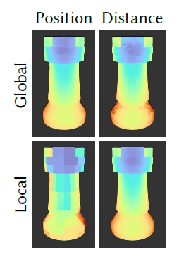
- Intersection point
- 备选:下图是结果的可视化,应该和上面的这个图一样
- 1D(到光线起点的 distance),3D(位置)
- locally(相对于 node 本身)、globally
- 尝试后,发现 locally+1D 效果好
- L1 Loss
- 解释:1D 的信号更好学习
- 备选:下图是结果的可视化,应该和上面的这个图一样
- Auxiliary intersection data
- 只有 normal+albedo
- the other BSDF parameters are fixed by the user
- 也就是说其他 BSDF 参数不能从网络中获取
- the other BSDF parameters are fixed by the user
- 实验发现
- albedo:relative L2 loss
- normal:L1 loss
- 只有 normal+albedo
- 2:实验发现重视 visibility 和 distance 更好
\[ L = 2L_{\text{visibility}}+2L_{\text{distance}}+L_{\text{normal}}+L_{\text{albedo}} \]
Level of detail
- 设置 multiple base-BVH cuts,每一个对应 LoD 的一个层级
- register a new LoD at regular training iteration intervals.
- 随机选择一个 tree-cut(对应一个 LoD)进行训练
实现
基础
- fully software-based CUDA wavefront path tracer
- tiny-cuda-nn
- half-precision scalars
- neural prefiltering 在 RTX 3080,其他都是 RTX 3090
细节
- BVH construction
- N-BVH 需要自己操纵,因此不能利用硬件加速
- CPU 建立,传到 GPU
- 网络
- batches size:\(2^{18}\)
- Adam optimizer
- lr:0.01
- MLP
- 4 hidden layers,64 neurons each
- ReLU
- 网络输出
- normal:linear activation
- 其他:sigmoid activation
- hash grid
- 8 levels:\(8^3\to1024^3\)
- 4 features per level
- 只通过修改 hash-map size 来调整网络大小
- BVH 边界很小的时候,可能受到浮点数误差的影响
- 之前工作可以减轻这个问题
应用
Hybrid Path Tracing
- 主要是起到压缩场景、减小显存开销的作用
- TLAS + BLAS
- each BLAS is either a classical BVH or our N-BVH
- 一般来说,一个 mesh 一个 BLAS
结果
- 一个示例:1920×1080
- 只压缩复杂的东西(棋子),棋盘格没有压缩
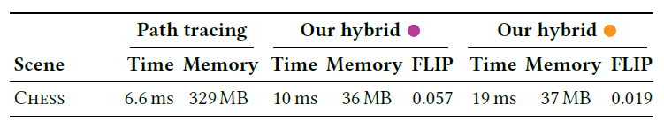
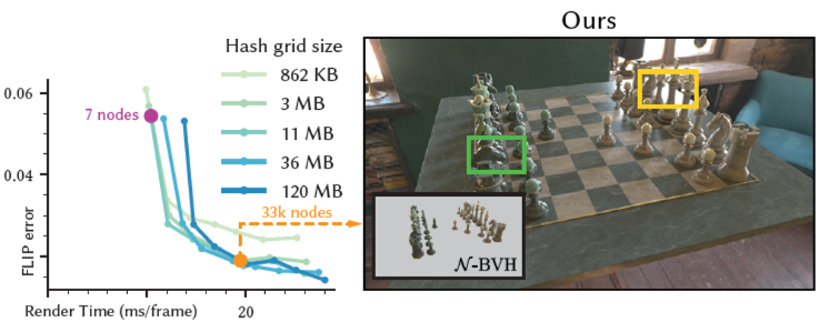
- Reconstruction quality & performance
- trade off
- render times & reconstruction quality
- 主要和 Neural Nodes 的数量相关,和 Hash Grid Size 相关性小一些
- trade off
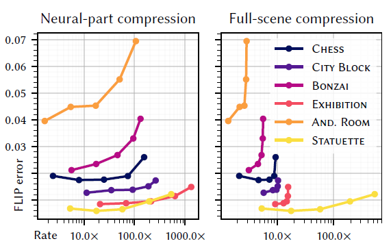
- Compression rate
- 通过调整 Hash Grid Size 来调整压缩率
- Neural Node 数:33k
- 因为有些东西不压缩,这里给了两个指标
- 最主要的压缩来源是 mesh 的简化
- 还放了一个 3D 扫描的 2.69G 的猛犸象
消融实验
- Hash-grid size vs. node count
- error 的主要影响因素:Neural Node 的数量
- memory footprint 的主要影响因素:hash grid size(可学习参数多)
- Training time
- 最影响训练时间(error)的也是 Neural Node 的数量
- 多了,traversal 的时间长了
- 最影响训练时间(error)的也是 Neural Node 的数量
- Hash-grid utilization
- mesh 分布稀疏的时候,hash grid 的优势体现出来了
Neural Prefiltering
- neural prefiltering 可以在感知 error 较低的情况下节省大量存储
- 这个暂时还没看,等到看完上面这个论文再说
讨论
Limitations
- assumption of convexity (or concavity) of the geometry inside a
neural node
- 当 Neural Node 比较少的时候,存在误差
- 局限:the fixed number of encoded points per node
- 适应性的分布 points 个数效果会更好
Future Work
- 泛化
- mesh 表示到任意可以求交点的表示
- dynamic geometry