(论文)[2005-WSCG] Go with the Winners Strategy in Path Tracing

Posted on 2023-11-14 Edited on 2023-12-06 In CG.Paper Views:

启发式决定 RR/S 系数，分析是基于全局的，但是实际上最后还是退化成了只依赖于 camera ray

GWTW

Go with the Winners Strategy in Path Tracing
- WSCG
- 2005

Introduction

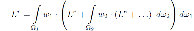
\(L^r\) ：the reflected radiance
\(L^e\)：the emission
\(w=\text{BRDF}\times\cos\)：the scattering density

论文：minimizes this total computation error and keeps the computational time low.

Previous work

Russian-roulette、Splitting、Joining
RR
- albedo：效果并不好
  - luminance of the albedo（spectral rendering）
  - 例如：先经过红色 (1,0,0) 表面、再经过绿色 (0,1,0) 表面，此时没有贡献，但是 albedo 无法识别
- throughput：效果比 fixed 要好
- fixed：场景 albedo 的平均值
window：\(W^{-},W^{+}\)

Random walks

Random walks with termination, splitting and joining
当前信息
- \(W^{l-1}\)
- \(l\) 点的材质信息

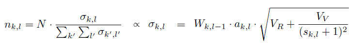
Splitting

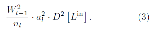
\(n_l>1\)

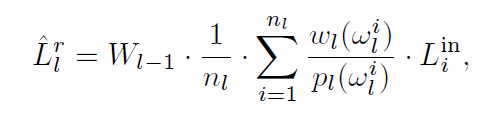
假定：采样 pdf 近似是零方差
- \(\dfrac{w_l}{p_l}=a_l=\text{const},\forall w_l\)
此时方差如下：这里的 \(D^2\) 是方差的记号

Random termination

\(n_l<1\)
假设不发射随机光线就能得到一个估计值（不一定无偏），使用 \(\Delta L\) 表示误差
- RR 的话，则直接返回 0（此时我们知道是 0，因此是无偏）

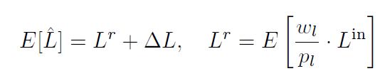
继续的话使用一个估计的为线性组合（下图红色部分）
- \(\alpha+\beta=1\)
此时总的估计如下

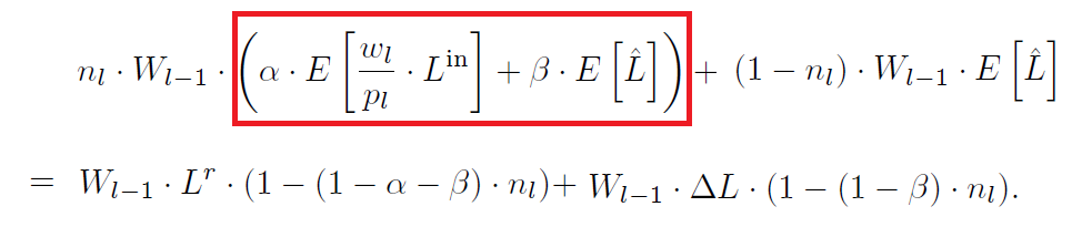
如何在加入有偏估计的同时，还能得到无偏的结果？
- 总的估计为 \(W_{l-1}\cdot L^{r}\) \(\Rightarrow\) 上面第二项为 \(0\) \(\Rightarrow\) \(\alpha=\dfrac{1}{n_l}\)
- 有偏估计存在期望即可
在无偏的条件下，方差如下
- 检验过没有问题：\(E=n_lE_1+(1-n_l)E_2\)（方差也是一个期望）

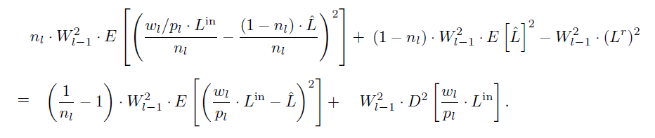
假定：\(\hat{L}\) 估计比较准
- \(\hat{L}\approx L^{r}\)
- 此时：\(E\approx D^2\)
在此假定下，方差如下

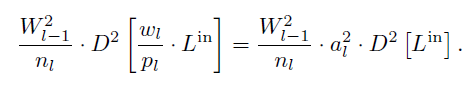
Estimation of D2

估计方差
方差来源
- 不同 \(\omega\)
- \(L^{\text{in}}(\omega)\) 本身是个估计
根据两个来源展开
- 依据：\(E[(X-a)^2]=E[(X-EX)^2]+(a-EX)^2\)
- 粉色期望：对 \(L^{\text{in}}\) 内部求期望（把 \(\omega\) 的部分展开了）
- 红色期望：对 \(\omega\) 和 \(L^{\text{in}}\) 内部求期望
- \(\tilde{L}^{\text{in}}(\omega)\)：\(L^{\text{in}}(\omega)\) 的真实值（没有内部方差）

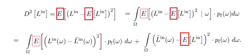
拆分之后
- 第一项：算法对于 \(L^{\text{in}}(\omega)\) 估计的准确程度
- 第二项：真实值 \(\tilde{L}^{\text{in}}(\omega)\) 在各个方向上的变化程度（方差），与采样算法无关
  - 如果是镜面，则为 0
  - 一般来说，反射叶越大，方差越大、
  - 近似：和反射叶的大小的平方成正比（只考虑 BRDF，不考虑光照）
第一项
- 使用一个全局的常数来表示：\(V_R\)
第二项
- Phong-like material，有一个 shininess 参数 \(s_l\) 控制反射叶的大小
  - specular：\(s=\infty\)
  - diffuse：\(s=0\)

\[ \dfrac{V_V}{(s_l+1)^2} \]

因此

\[ D^2[L^{\text{in}}]=V_R+\dfrac{V_V}{(s_l+1)^2} \]

Variance-cost optimization

计算开销：\(n\) rays
总体目标：在计算开销相同的条件下，最小化方差
方差：所有光线、所有中间节点的方差
- \(k\) light rays
- \(l\) bounces

\[ \sum_{k}\sum_{l}\dfrac{\sigma_{k,l}^2}{n_{k,l}} =\sum_{k}\sum_{l}\left(W^2_{k,l}\cdot a^2_{k,l}\cdot\left(V_R+\dfrac{V_V}{(s_l+1)^2}\right)\right) \]

限制条件：\(\sum n_{k,l}=N\)
拉格朗日乘子法

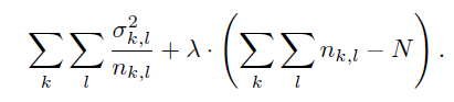
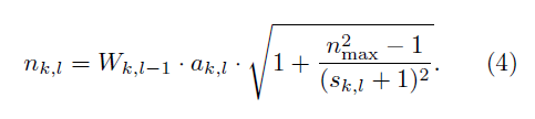
结果如下

我们只需要使用正比的性质即可，如下是一种可行方案
- pure specular：\(s_l=\infty\Rightarrow n_l=1\)
- pure diffuse：\(s_l=1\Rightarrow n_{\max}\)
  - \(n_{\max}\) 的选择与场景性质有关，例如光照相关
    - 光照各向同性：\(n_{\max}=1\)
    - 光照各向异性：\(n_{\max}\uparrow\)
  - 文章实现：\(n_{\max}=10\)
- 如果具有多种材质，则将其分开（specular + diffuse）
结论

GWTW

Variance based Go with the Winners Strategy
根据上面的式子4计算系数
- \(<1\)：RR
- \(>1\)：S（四舍五入）
实现上还加上了有偏估计 \(\hat{L}\)

估计获取

[WSCG-2003] Variance reduction for russian-roulette.
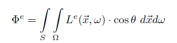
因为加了 NEE，因此只需要考虑 reflected radiance
场景是 closed 的，光源发射的 power/flux 如下

场景平均 albedo = \(\tilde{a}\)，此时总的反射的 power 如下
- average power

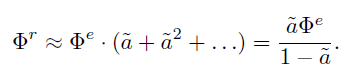
平均 \(\hat{L}\) 估计如下（average radiance）

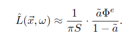
为什么 \(/S\pi\)？
- 假设 \(\hat{L}(\vec{x},\omega)\) 对任意 \(\omega\) 都相同，根据定义有如下式子（\(H^2\)：半球面）

\[ \begin{aligned} \text{Irradiance}&=\dfrac{\text{Power}}{\text{Area}}=\dfrac{\Phi^{r}}{S}\\ &=\int_{H^2}\hat{L}(\vec{x},\omega)\cos\theta\;\mathrm{d}\omega\\ &=\hat{L}\int_{H^2}\cos\theta\sin\theta\;\mathrm{d}\omega\\ &=\hat{L}\int_{0}^{2\pi}\left(\int_{0}^{\pi/2}\cos\theta\sin\theta\;\mathrm{d}\theta\right)\;\mathrm{d}\phi\\ &=\hat{L}\pi \end{aligned} \]

于是有 \(\dfrac{\Phi^{r}}{S}=\hat{L}\pi\Rightarrow\hat{L}=\dfrac{\Phi^{r}}{\pi S}\)

实验对比

方法
- PT with classical RR（local albedo based RR）
  - 这个也并不公平，应该比 throughput based RR
- GWTW（论文方式）
条件
- the same number of rays
  - 实际上这个条件并不等于开销一致，GPU 上实现 splitting 存在 divergence 问题
- NEE
结果
- 论文说 GWTW 实现快了 \(20\%\)，解释是减少了递归调用
  - 太神奇了，不过论文的结果在实现上，看上去 CPU 实现的
- GWTW 达到相同的 error，可以减小 \(30\sim50\%\) 的光线

总结

RR、S 的方差统一形式的表达归功于
- 个性
  - S：加入了估计项，而且假定 \(\hat{L}\approx L^{r}\)
- 共性
  - 近似：\(p(\omega)\propto w_l\)（这个能够实现，BSDF 采样即可）
进一步的近似：材质的近似
实现很快：CPU 实现，splitting 的劣势没有显现出来
实际上还是退化成了只依赖于 camera ray