(论文)[2016-SIG] Adjoint-Driven Russian Roulette and Splitting in Light Transport Simulation
ADRRS
贡献
- 将 RR 和 Splitting 结合到一个统一的框架里(RRS)
- 通过路径的 total expected contribution 来决定 RRS 系数
- thoughput
- pre-computed irradiance
Introduction
- 传统
- RR,基于
- local surface reflectivity
- accumulated path weight (a.k.a. throughput)
- Splitting,基于
- heuristics based on local BRDF roughness
- local 的特征容易实现,但是效果不好
- RR,基于
- 问题:忽略了真实分布
- actual distribution of light
- visual importance
- ex:暗表面长路径
- local surface based RR:会被过早截断
- 复杂可见性、参与介质场景中常见
- 本文:根据路径的 total expected contribution 来决定 RRS
系数
- path weight \(\times\) adjoint transport solution(预计算保存在场景中)
Related Work
- Particle transport
- analog:根据物理的概率来决定 collisions、absorption、scattering,所有的粒子都等价
- non-analog simulations:修改概率,提高效率
- RR+S
- throughout based:不考虑 expected future behavior
- Importance sampling
- Adjoints:TODO
- Path guiding
- Weight window
- increases robustness
- RR and splitting are combined in one variance reduction tool called the weight window
- 当 weight 小于/大于 weight window 时使用 RR/S,从而使得 weight 保持在 window 内部
- Booth and Hendricks [1984]
- 让 window 的中心 inversely proportional to 重要性函数(让重要的地方粒子更多)
- Go-with-the-winners
- Szirmay-Kalos and Antal [2005]
- efficiency analysis:基于 local material properties、scene dependent parameters
- Szirmay-Kalos and Antal [2005]
Background
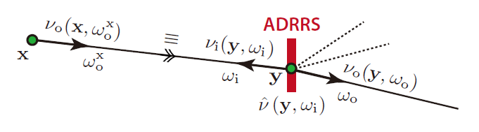
- particle tracing / unidirectional path tracing
- MC 估计:weight \(\times\) radiance
- \(\text{i}=\text{incident}\)
- 在位置 \(\mathrm{y}\)
反射之后的出射权重
- \(\text{o}=\text{outgoing}\)
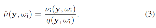
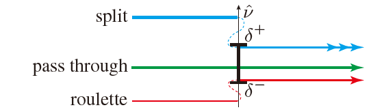
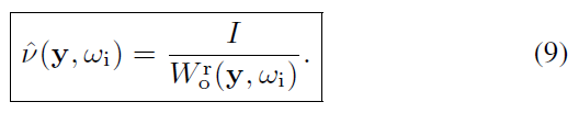
- \(\hat{\nu}\):在应用了 RRS 之后的 weight
- 文章中的 \(\omega_o\) 指向 quantity 传输的方向
![]()
- Russian roulette and splitting
Adjoint-Driven RR and Splitting
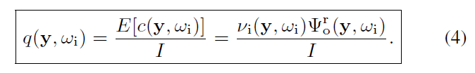
Unified Russian Roulette and Splitting
- RRS
- \(q<1\):RR
- \(q>1\):S(非整数情况后面说明)
- 示意图,所有新生成的粒子 \(\hat{\nu}\) 相同
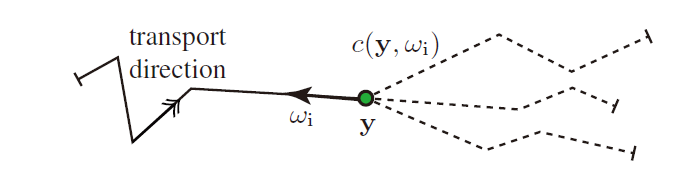
Determining the RRS Factor
- 让 \(q\) 正比于期望的贡献值
- 直观的,当达不到期望贡献值时,则倾向于停止
- 理论在 weight invariant 部分
- \(\Psi\) 的含义
- light subpath:visual importance \(W\)
- camera subpath:radiance \(L\)
- 这里不考虑自发光,因为我们只在意 \(\mathrm{y}\) 处的 scatter 的能量的期望值
- 合理的,自发光 RRS 不管是多少,结果都是一个精确值,不受影响
\[ \Psi^{\text{r}}=\Psi-\Psi^{\text{e}} \]
- \(c(\mathrm{y},\omega_\text{i})\)
的可视化
- 注意每一条虚线都是对 \(\Psi^{\text{o}}\) 的无偏估计
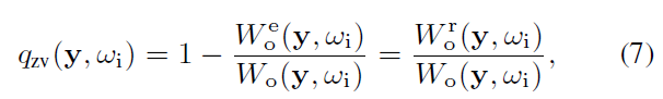
Weight Invariant in ADRRS
- 设计的时候,保证如下不变量
- which holds for particle weight in a zero-variance (ZV)
scheme
- 具体见附录
- which holds for particle weight in a zero-variance (ZV)
scheme
Algorithm
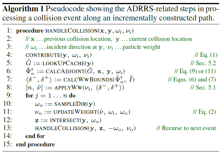
- 计算 RRS 系数 \(q\) 需要 \(I,\Psi\)
- 我们对 \(I,\Psi\) 进行近似估计
- 因为近似存在偏差(不够准确),weight window 用于修正
Weight Window
- 放松 RRS(在 RRS 执行之前留有余地),提高鲁棒性
- 放松 \(\hat{\nu}\) 的限制,保证 \(\hat{\nu}\in[\delta^{-},\delta^{+}]\) 即可,而不是 \(\hat{\nu}=C_{\text{ww}}\)
- 保证权重 \(\hat{\nu}\)
都在设置的范围内
- \(\nu_i\in[\delta^{-},\delta^{+}]\):不变 \(\Longrightarrow\) \(\hat{\nu}=\nu_i\)
- \(\nu_i>\delta^{+}\):split,\(q=\dfrac{\nu_i}{\delta^{+}}\Longrightarrow\hat{\nu}=\delta^{+}\)
- \(\nu_i <\delta^{-}\):RR,\(q=\dfrac{\nu_i}{\delta^{-}}\Longrightarrow\hat{\nu}=\delta^{-}\)
- split 的非整数情况
- 概率 \(\lfloor{q}\rfloor+1-q\) 发射 \(\lfloor{q}\rfloor\) 条光线
- 概率 \(1-\lfloor{q}\rfloor+q\) 发射 \(\lfloor{q}\rfloor+1\) 条光线
- window center 设置为式子 5
的值
- 具体如何计算后面说
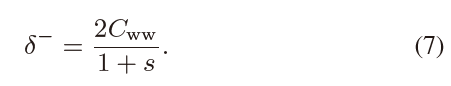
\[ \dfrac{\delta^{-}+\delta^{+}}{2}=C_{\text{ww}}=\dfrac{\tilde{I}}{\tilde{\Psi}_{\text{o}}^{\text{r}}(\mathrm{y},\omega_\text{i})}\qquad(6) \]
- 推荐设置
- \(\delta^{+}=s\delta^{-}\)
- \(s=5\)
- 早期一些核科学研究的推荐设置
- 此时可以得到
- 在 weight window 之后,我们还会对 \(q\) 加上 clamp
- 很小的 RRS 系数会导致大方差(估计不准)
- RR 必然带来方差的增大
- 很小的 RRS 系数会导致大方差(估计不准)
- weight window 相当于是给 \(\hat{\nu}\) 做了 clamp
Adjoint Solution Estimate
- \(\tilde{\Psi}_{\text{o}}^{\text{r}}(\mathrm{y},\omega_\text{i})\)
- 之前
- photon/importon density estimate:慢而且不准
- spatial-directional distribution
- 我们:无方向的缓存,而且鲁棒
- \((a)\) 就是我们的方法
- \((b)\) 加上了 path guiding
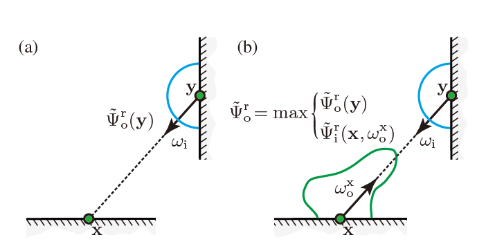
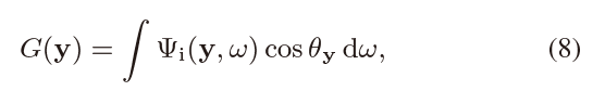
- 预训练 irradiance(/diffuse visual importance)\(G\)
- adjoint 的估计
- \(\kappa(\mathrm{y})\):total material reflectivity(albedo)
- \(\dfrac{\kappa(\mathrm{y})}{\pi}\):Lambert 漫反射的 BRDF
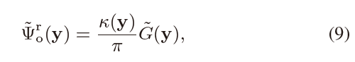
- 为什么是上面的表达形式
- 在方向上做平均(Lambert)
- \(\Psi^{\text{r}}_{\text{o}}(\mathrm{y},\omega_i)=\Psi^{\text{r}}_{\text{o}}(\mathrm{y})\)
- 在方向上做平均(Lambert)
\[ \begin{aligned} \Psi^{\text{r}}_{\text{o}}(\mathrm{y}) &=\int_{\Omega}\Psi_{\text{i}}(\mathrm{y},\omega)\dfrac{\kappa(\mathrm{y})}{\pi}\cos\theta_{\mathrm{y}}\;\mathrm{d}\omega\\ &=\dfrac{\kappa(\mathrm{y})}{\pi}{\color{red}\int_{\Omega}\Psi_{\text{i}}(\mathrm{y},\omega)\cos\theta_{\mathrm{y}}\;\mathrm{d}\omega}\\ &=\dfrac{\kappa(\mathrm{y})}{\pi}{\color{red}G(\mathrm{y})}\\ \end{aligned} \]
- 预计算:Vorba 2014(On-line learning
of parametric mixture models for light transport simulation)
- 和他不一样的地方,我们双向追踪光线,构建 \(\tilde{G}\) 的估计(irradiance/diffuse visual importance)
- Vorba:fit directional distributions
- EARS 对于预计算的实现:空间划分做累计和(类似 PPG)
- 细节:借鉴 Vorba(细节看论文)
- 当 \(\tilde{G}\)
无法获得的时候,使用 kernel density estimation 从临近的粒子中获取一个
estimate
- 每一个粒子都带有一个半径(最深的最大),同时让光场快的地方更密集
- 每一轮迭代使用 progressive kernel density estimation 更新 \(\tilde{G}\),同时计算 rel-error \(\dfrac{\text{stddev}(\tilde{G})}{\tilde{G}}\)
- ADRRS 只有在 rel-error < 30% 的时候使用,否则使用一个全局固定的 large weight window
- smoother:周围的缓存做平均
- 当 \(\tilde{G}\)
无法获得的时候,使用 kernel density estimation 从临近的粒子中获取一个
estimate
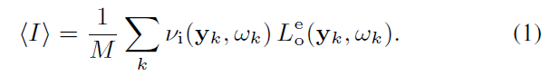
Measurement Estimate
- \(\tilde{I}\):EARS 中使用降噪后的结果
- 之前
- 使用一个常数,而不是 \(\tilde{I}\),使得在一次 collision 的时候,particle 的权重恰好落在区间中心
- camera ray
- 实际实现上,使用记录的缓存用于更新
- 发射 4 条 jittered primary rays,查询 irradiance
- diffuse/glossy:碰到即返回
- specular:继续
- 10 条还没碰到,则在 10th 处查询
- light ray
- 已经获得的结果,所有像素的平均值(因为我们不知道会被贡献给哪一个像素)
Path Sampling Algorithm
- First Collision
- camera ray:第一次 RRS 系数 \(q=1\)
- 第一次使用只会用于降低像素内的方差,这通常很小
- Why
- 第一次使用只会用于降低像素内的方差,这通常很小
- light ray:第一次也能发生
- camera ray:第一次 RRS 系数 \(q=1\)
- 避免 ray tree 太大
- RRS <= 100
- 每一条路径上的最大分裂次数 <= 1000
- RRS 累乘
- NEE:对每一条分裂的 ray 做 NEE
- \(q\) pairs
Combining ADRRS with Path Guiding
- Vorba 14
- classic RR 可能会去除 Path Guiding 的效果
- \(\delta^{-}=1\mathrm{e}^{-6}\) 设置很小,效果并不好,失去 RR 的意义了
- 引入 splitting,当 weight > 2 original value 时使用 splitting,同时设置 \(s=2\times10^{6}\)
- 我们
- 基于 Vorba 14,同时预计算 \(\tilde{G}\) 和 directional sampling
distribution
- 训练的时候也加入 ADRRS
- 进一步的,我们利用 distribution 构建更好的 adjoint
- 基于 Vorba 14,同时预计算 \(\tilde{G}\) 和 directional sampling
distribution
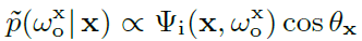
- 利用 distribution 估计 adjoint \(\tilde{\Psi}_{\text{o}}^{\text{r}}(\mathrm{y},\omega_\text{i})\)
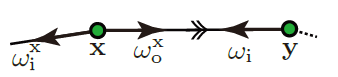
- 利用前一个点 \(\mathrm{x}\) 进行估计
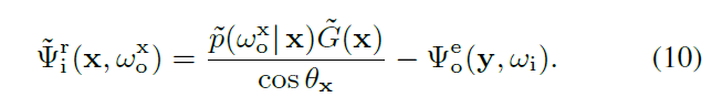
- 根据 PG 的 ZV 估计设计要求(\(\tilde{G}(\mathrm{x})\) 做归一化),有如下式子,推导得到式子 10
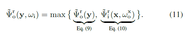
- 根据式子 10 和之前式子 9,得到实际使用的 adjoint 估计(式子 11)
- 取 \(\max\),则 \(C_{\text{ww}}\) 越小,则停止的光线数越少(\(\delta^{-}\) 也小了),避免方差太大(glossy 场景)
ADRRS and Zero-Variance Schemes
- zero variance (ZV)
- ZV 条件下,推导得到 \(\mathrm{y}\)
处的 \(q\) 如下,具体过程见附录
- 前一个点 \(\mathrm{x}\)
- ZV 下

- 这样得到的 \(q\) 和 \(\mathrm{x}\) 之前的情况都无关(不包含 \(\tilde{v}\) 项)
- RRS as importance sampling
- 这样子的 \(q\),好像是一种重要性采样
- 实际 pdf 比零方差高了,就使用 RR,减小采样;低了,就使用 S,增加样本
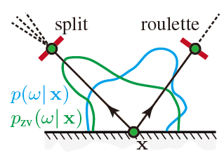
- Residual variance
- RR 下,等价于拒绝采样(rejection sampling)
- splitting 不能降低 \(\mathrm{x}\) 出的方差,因为其发生在 \(\mathrm{y}\)
- 因此如果 pdf 很差,ADRRS 起到的补救作用很小
- 光路:diffuse wall -> spacular-like floor -> light
- diffuse 的 pdf 很差,则 floor 的 splitting 补救作用很小
- Zero-variance sampling
- ZV scheme:\(p(\omega\mid\mathrm{x})=p_{\text{zv}}(\omega\mid\mathrm{x}),\forall\omega\)
- 如此可以获取 ZV 的 \(q=q_{\text{zv}}=1\)
- 理解:pdf 是 ZV 了,就不需要 RRS 了
- 不同点
- PG:\(\mathrm{x}\) 点的估计是 ZV 的
- ADRRS:\(\mathrm{y}\) 处的方差降低了
- Path guiding methods
- pdf 越接近 ZV,则就不需要 RRS 了
- 否则,RRS 用于弥补 pdf 的偏差
Result
- 1 hour on an Intel Core i7-2600K CPU using 8 logical cores.
- training time included
- max bounces:40
- indirect light dominated scene
Limitation, Discussion, and Future Work
- Inaccurate adjoint and measurement estimates
- Efficiency-driven RR and splitting
- Splitting and combined estimators
- with BDPT
- Participating media
sup
transport
- radiance transport
- 分母:归一化(分子的积分)
- \(\mathrm{x}\):发射,\(\mathrm{y}\):收集
![]()
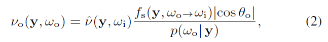
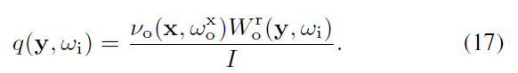
- visual importance transport
- 分母:归一化
![]()
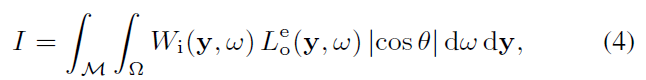
- light tracing
- 估计如下
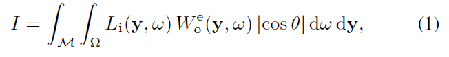
- 可以看 PT 的 MC 估计,相当于此时的权重函数为 \(L\),此时收集的 transport 为 \(W\)
- \(\mathcal{M}\):全表面空间
- 想象一个像素是一个小 patch,到达/出去这个 patch 的 flux 定义如下
- \(W\):这个 patch 直接可见的点及其方向 \(\Rightarrow\) 1
- \(L\):radiance
- flux:垂直,需要乘 \(\cos\)
- 也就是说这里的 \(I\) 指的是通量 flux
- 估计如下
- path tracing
- 估计如下
采样
- 出射采样,以 light tracing 为例,配套的估计是 visual importance transport
- emission:首先采样一个光源
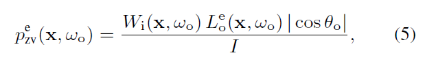
- scatter:发生散射的地方,出射方向的概率正比于总出射 \(L\)
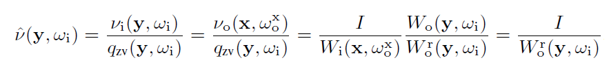
Light Tracing 证明
- survival probability
- 这样的设计,能够让路径只有在相机处恰好完全终止(相机不与 visual importance 交互)
- 证明如下式子
- 已知
- 采样是 ZV 的,包括 light ray/camera ray
- 对称性
- 红色:radiance transport
- 分类讨论:主体思路,数学归纳法证明
emission
- 注意光源不散射,除了发光外不与光线交互
- RRS 前
- 按照正比发射:\(p=\dfrac{WL\cos}{I}\)
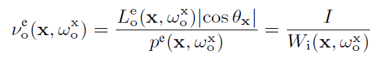
- RRS 后
- RRS 的 ZV 定义(式子 7)+ RRS 前系数
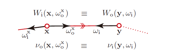
中间节点
- \(\mathrm{x}\):发射,\(\mathrm{y}\):收集
- 归纳法,假设 \(\mathrm{x}\) 满足要求
- RRS 前
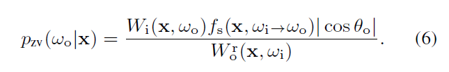
- 在 \(\mathrm{x}\) 处散射
- 根据式子 6,此时 \(L\) 变为 \(\hat{v}f_\text{s}\)
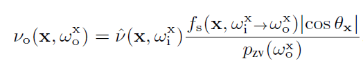
- 归纳
\[ \hat{v}(\mathrm{x},\omega_{\text{i}}^{\text{x}})=\dfrac{I}{W_{\text{o}}^{\text{r}}(\mathrm{x},\omega_{\text{i}}^{\text{x}})} \]
- 此时能够得到
- \(\nu=\dfrac{\hat{\nu}f_{\text{s}}\cos}{p}=\dfrac{I}{W_{\text{o}}}\cdot f_{\text{s}}\cos\cdot\dfrac{W_{\text{o}}}{W_{\text{i}}f_{s}\cos}=\dfrac{I}{W_{\text{i}}}\)
- RRS 后的推导和 emission 一样,于是得到 \(\mathrm{y}\) 也满足结果
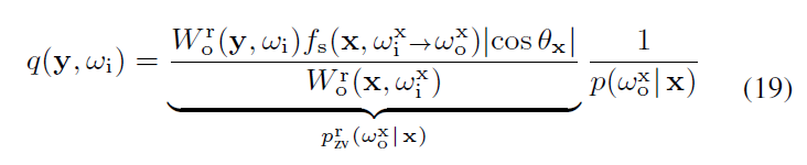
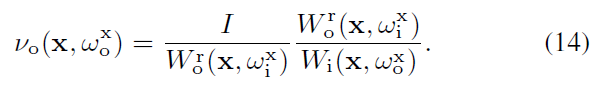
PG
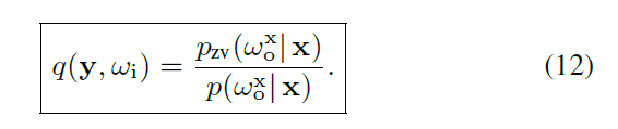
- 原始论文中式子 12 的证明
- 当前点 \(\mathrm{y}\) 的 RRS 系数由前一个点 \(\mathrm{x}\) 的采样 pdf 和 ZV pdf 决定
- 更一般的版本:\(p^{\text{r}}_{\text{zv}}\) 代替 \(p_{\text{zv}}\)(不包含 emission,这样在
emission 处也正确)
- 都替换成 \(X^{\text{r}}\) 就行
证明
- 定义
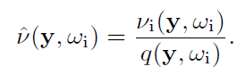
- 对称性 + 上面的证明 \(\hat{v}(y)\)
- transport
![]()
- 上面的证明 \(\hat{\nu}(x)\)