(论文)[2017-EGSR]Practical Path Guiding for Efficient Light-Transport Simulation
PPG
概述
PPG
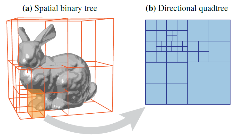
- SD-Tree:空间二叉树 + 方向四叉树
- 3D spatial domain of the light field
- 2D directional domain
- 每一个二叉树的叶子节点都包含一个四叉树
- 优点:容易集成到 PT 框架里
- 算法启发:path guiding 算法和复杂算法相比同样有效
- 其他贡献:固定时间,找到最合适的训练时间/渲染时间分配
其他算法
其他方法
- constructing high-energy light paths
- BDPT:Bi-directional path tracing
- MLT:Metropolis light transport
- offsetting the inefficiency by reusing computation
- PM:Realistic Image Synthesis Using Photon Mapping
- Instant radiosity
- VCM:Light transport simulation with vertex connection and merging
- A path space extension for robust light transport simulation
- Gradient-domain path tracing
- PM:Realistic Image Synthesis Using Photon Mapping
- constructing high-energy light paths
其他存储方式
- spatially cached histograms:Importance driven path tracing using the photon map
- cones:Importance sampling with hemispherical particle footprints
- gaussian mixtures model(GMM):On-line learning of parametric mixture models for light transport simulation
介绍
- guiding 的概念
- Importance driven path tracing using the photon map(histograms)
- A 5d tree to reduce the variance of monte carlo ray tracing(5D tree)
- path guding 的改进
- Global Importance Sampling of Glossy Surfaces Using the Photon Map(discretized BSDF、caustics)
- Importance sampling with hemispherical particle footprints(cones、irregular)
- On-line learning of parametric mixture models for light transport simulation(gaussian mixtures)
- Product Importance Sampling for Light Transport Path Guiding(和 BSDF 一起重要性采样)
- Adjoint-driven russian roulette and splitting in light transport simulation
- Learning light transport the reinforced way(结合训练+渲染)
- PPG
- adjoint-based Russian roulette
- progressive reinforcement learning
- fusing the rendering and learning algorithms into one
- 每一个 pass 都是 unbiased
- 混合存储表示
- Volume-Surface Trees
- Rasterized bounding volume hierarchies
- spatial octree and a directional kd-tree:Spatial directional radiance caching
算法
- two SD-trees
- one for guiding the construction of light paths
- another for collecting MC estimates of incident radiance
- double the number of samples across iterations
- 近似渲染方程中的 \(L(x,\omega)\) 项
- incident radiance field
\[ L_{o}(x, \omega_{o})=L_{e}(x, \omega_{o})+\int_{\Omega} L_{i}(x, \omega_{i}) f_{r}(x, \omega_{i}, \omega_{o})(n \cdot \omega_{i}) d \omega_{i} \]
收集 L
- 对得到的光路的每一个顶点做收集
- 顶点 \(v\):\[L(x_v,\omega_v)\]
- binary tree
- 找到包含 \(x_v\) 的叶子节点,记录 \(L\)
- quadtree
- 继续向下搜索,进入包含 \(\omega_v\) 的叶子节点,在这些节点上都记录 \(L\)
- pdf over all leaf node in quadtree
空间二叉树
- 选择
- 交替使用 \(x,y,z\) 轴
- always split the node in the middle
- 细化
- 如果一个叶子节点的计数(\(L\)
记录次数)大于等于 \(c\cdot\sqrt{2^k}\),则分裂
- \(k\):迭代轮次
- \(2^{k}\) 正比于发射的光线数目
- \(c\):二叉树的分辨率、四叉树的收敛率相关
- 分裂的时候,计数平均分给两个子节点
- 如果一个叶子节点的计数(\(L\)
记录次数)大于等于 \(c\cdot\sqrt{2^k}\),则分裂
- 每一个的叶子节点的计数 \(\approx c\cdot\sqrt{2^k}\)
- 叶子节点的数量正比于 \(\dfrac{2^k}{c\cdot\sqrt{2^k}}=\dfrac{\sqrt{2^k}}{c}\)(一条光线,\(d\) 个记录,\(d\) 稳定)
- \(c\) 的确定
- \(s\):quadtree
每一个树节点的期望样本数
- 根据 quadtree 的拆分规则,每一个叶子节点采样概率基本接近(flux 接近)
- 单个 quadtree:\(s=\dfrac{S}{N_l}=\dfrac{总样本数}{叶子节点数}\)
- 根据 \(S\approx
c\cdot\sqrt{2^k}\),可以得到
- 实验测试,\(N_l\approx300\)
- \(s=40\) 收敛效果就已经不错了
- 初始设置 \(c\)(\(k=0\))
- \(s\):quadtree
每一个树节点的期望样本数
\[ c\approx\dfrac{S}{\sqrt{2^k}}=\dfrac{s\cdot N_l}{\sqrt{2^k}}=12000 \]
方向四叉树
- 每轮迭代结束之后都重建,更好地反映 flux 分布
- 目的:根据上一轮收集的 flux, 每个节点的收集的 flux 都不超过 \(\rho=1\%\)
- 当前节点/根节点
- 初始化
- 存在:上一轮的迭代结果
- 新生成:父节点的 quadtree
- 从根节点开始,对于叶子节点,如果超过 \(1\%\),则展开这个节点,把这个节点的 flux
均分给子节点
- 递归进行
- 内点则可以剪枝(\(<1\%\) 则子节点必然 \(<1\%\))
- 结果:Spherical regions with high incident flux are thus represented with higher resolution
训练与渲染
- 序列:\(\hat{L}^{1},\hat{L}^{2},\cdots,\hat{L}^{M}\)
- \(\hat{L}^{1}\):BSDF sampling
- \(L^{k}(k>1)\):BSDF + \(\hat{L}^{k-1}\)(MIS)
- 采样过程:路径节点 \(v\)
- 找到包含 \(x_v\) 的叶子节点,获得 quadtree
- 采样策略:Probability trees
- 按照记录的 flux 进行采样
样本数
- 每轮迭代 \(\times2\)
- 平衡训练与渲染
- 每轮都相同,为 \(s\)
- 则每次只有 \(s\) 个样本用于图像生成,\(ks\) 的都是用于训练
- \(\times2\)
- 则每次有 \(2^k\) 个样本用于图像生成,\(2^{k+1}-2\)
- 每轮都相同,为 \(s\)
- 让到达叶子节点的采样数类似
- 分裂叶子节点数 \(\times2\)
- 样本数 \(\times2\)
渲染
- 只使用当前迭代轮的样本
- unbiased:样本之间是独立的
- 最终视频展示:当 \(k\) 轮的 path 样本数高于 \(k-1\) 轮时,替换展示图
平衡训练与渲染
compute budget
- 总预算(budget):\(B\)
- \(B\) 的选择:样本数、时间
- define the budget to unit variance:\(\tau_k=V_k\cdot B_k\)
- \(I_k\):第 \(k\) 轮迭代生成的图片
- \(V_k\):\(I_k\) 的 mean variance of pixels
- \(B_k\):构建 path 的开销
- \(\hat{B}_k\):剩余预算
\[ \hat{B}_k=B-\sum_{i=1}^{k-1}B_k \]
- 最终图的方差估计
\[ \hat{V}_k=\dfrac{\tau_k}{\hat{B}_k} \]
- 目标:找到最小的 \(\hat{k}\),使得最小化最终的方差
\[ \hat{k}=\mathop{\arg\min}_{k}\hat{V}_k \]
- 假设:\(\tau_k\) 单调递减 + 凸函数
- 此时能够推出 \(\hat{V}_k\) 也是凸函数(证明有问题,见附录)
- 于是只需要找到最小的 \(k\) 满足 \(\hat{V}_{k+1}>\hat{V}_k\) 即可(多计算一次,但是是值得的)
- 如果缺少了凸函数的保证,则找到的结果只是一个局部最优
target variance
- 类似方法
- 渲染预算:\(\bar{B}_k\)
- 目标方差:\(\bar{V}\)
- \(\bar{B}_k\) 的估计 \(\dfrac{\tau_k}{\bar{V}}\)
- 总预算
\[ \tilde{B}_k=\bar{B}_{k}+\sum_{i=1}^{k-1}B_i \]
- 找到 \(\hat{k}\)
\[ \hat{k}=\mathop{\arg\min}_{k}\tilde{B}_k \]
- \(B_k\)
单调递增,且是凸函数(样本加倍)
- 只需要找到 \(\tilde{B}_k>\tilde{B}_{k-1}\) ,训练停止
- 直观理解,花了更多时间,但是不能够获得期望的方差减小收益
\[ \begin{aligned} \tilde{B}_k&=\bar{B}_{k}+(\tilde{B}_{k-1}-\bar{B}_{k-1})+B_{k-1}\\ &=\tilde{B}_{k-1}+(\bar{B}_{k}-\bar{B}_{k-1})+B_{k-1} \end{aligned} \]
实验结果
- equal time
- GMM/SD-Tree 都是不使用 NEE 的(加强对比)
- GMM 的预训练时间不算入(说明我们更好)
- 不加 importance sampling(正交的,都可以加)
场景
- TORUS
- very long chains of specular interactions
- a significant amount of specular-diffuse-specular (SDS) light transport
- POOL
- difficult SDS light transport
- KITCHEN
- various glossy materials
- complex geometries
分析
Convergence
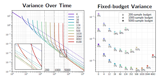
- 左图:不同的线表示使用不同的样本数进行训练
- 每轮迭代使用的样本数加倍
- 每轮增加:4、8、16、32、……
- 每轮总共:4、12、28、60、……
- 延长线:收敛率,使用当前分布继续渲染
- 每轮迭代使用的样本数加倍
- 右图:固定样本数,在左图中作 \(x=\text{samples}\),得到的交点
- 不同的点类型表示总预算(总样本数)不同
Memory Usage
- 根据展开原则,叶子节点数不小于 \(\dfrac{1}{\rho}\)
- 上限无界
- 实现中设定最大深度为 20
- quadtree 节点数上限:\(20\cdot\dfrac{4}{\rho}\)
- 最差情况下,叶子节点都是刚分裂形成的,流量 \(\ge \dfrac{\rho}{4}\)
- 因此叶子节点数 \(\le\dfrac{4}{\rho}\)
- 每一层的节点数肯定都小于总的叶子节点数:\(\le20\cdot\dfrac{4}{\rho}\)
- 实际测试
- \(\rho=0.01\Rightarrow \text{max-node}=8000\)
- 平均:300
- 最大:792
- SD-Tree 的存储:只需要保存最新的两棵树 \(\hat{L}^{k},\hat{L}^{k-1}\)
- spatial 只需要保存一棵树,每个叶子节点包含两个 quadtree
- 相当于只是更新了
- 测试:整个分布 \(<20\text{mb}\)
讨论
- directional quadtree distributions
- 当前:world-space-aligned cylindrical coordinates
- 其他:hemispherical
- 优点:不需要判别、很容易扩展到 volume path tracing
- 当前:world-space-aligned cylindrical coordinates
- quadtree
- 其他:Gaussian Mixture Model
- 随着空间位置变化大
- 不一定能找到全局最优
- 优点:increased robustness
- 其他:Gaussian Mixture Model
- temporal path guiding
- 容易扩展,增加一个维度 \(t\) 就行
- 采样策略
- MIS with BSDF sampling
- 改进
- ignore quads in the bottom hemisphere
- Portal-masked environment map sampling
- Importance resampling
- ignore quads in the bottom hemisphere
- 直接对乘积采样
- BSDF and the incident radiance
- Product Importance Sampling for Light Transport Path Guiding
- BSDF and the incident radiance
- Importance sampling spherical harmonics
- incident radiance distributions 转化为 Haar wavelets
- BSDF 使用 spherical harmonics 表示
- 开 NEE
- 集成到复杂框架中:对 BDPT、VCM 也有好处
- On-line learning of parametric mixture models for light transport simulation
附录
凸函数证明
- \(\hat{V}_k\) 凸函数性质证明
- 只要证明
\[ 2\hat{V}_k\le\hat{V}_{k+1}+\hat{V}_{k-1} \]
- 等价
\[ \begin{aligned} &\dfrac{2\tau_k}{\hat{B}_k}\le\dfrac{\tau_{k+1}}{\hat{B}_{k+1}}+\dfrac{\tau_{k-1}}{\hat{B}_{k-1}}\\ \Leftrightarrow\quad& 2\tau_k\le\dfrac{\hat{B}_k}{\hat{B}_{k+1}}\tau_{k+1}+\dfrac{\hat{B}_{k}}{\hat{B}_{k-1}}\tau_{k-1}\\ \end{aligned} \]
- 如果下式成立,则上式成立
- 凸函数:\(2\tau_k-\tau_{k-1}\le\tau_{k+1}\)
\[ \begin{aligned} &2\tau_k\le\dfrac{\hat{B}_k}{\hat{B}_{k+1}}(2\tau_k-\tau_{k-1})+\dfrac{\hat{B}_{k}}{\hat{B}_{k-1}}\tau_{k-1}\\ \Leftrightarrow\quad& 2\tau_k\le2\tau_k\dfrac{\hat{B}_k}{\hat{B}_{k+1}}+\left(\dfrac{\hat{B}_{k}}{\hat{B}_{k-1}}-\dfrac{\hat{B}_{k}}{\hat{B}_{k+1}}\right)\tau_{k-1}\\ \end{aligned} \]
- 因为有 \(\tau_k<\tau_{k-1}\),则下式成立即上式成立
\[ 2\tau_k\le2\tau_k\dfrac{\hat{B}_k}{\hat{B}_{k+1}}+\left(\dfrac{\hat{B}_{k}}{\hat{B}_{k-1}}-\dfrac{\hat{B}_{k}}{\hat{B}_{k+1}}\right)\tau_{k}\\ \]
\[ 2\le\dfrac{\hat{B}_{k}}{\hat{B}_{k-1}}+\dfrac{\hat{B}_{k}}{\hat{B}_{k+1}}\\ \]
- 转化为只含有 \(\hat{B}_k\) 之后,利用 \(B_k\) 单调递增性质(样本加倍)
\[ 2\le\dfrac{\hat{B}_{k}}{\hat{B}_{k}+B_{k-1}}+\dfrac{\hat{B}_{k}}{\hat{B}_{k}-B_k}\\ \]
- 等价于
\[ B_{k-1}-B_{k}-\dfrac{2B_{k-1}B_{k}}{\hat{B}_k} \]
ERROR
- \(\hat{B}_k\) 递减
\[ \hat{B}_k=\hat{B}_{k-1}-B_{k-1}<\hat{B}_{k-1} \]
\[ \dfrac{\hat{B}_{k}}{\hat{B}_{k-1}}-\dfrac{\hat{B}_{k}}{\hat{B}_{k+1}}<0 \]
- 于是 \(\tau_k<\tau_{k-1}\) 这一步转换有问题
观点
- 其他有趣论文
- Gradient-domain path tracing
- On-line learning of parametric mixture models for light
transport simulation
- gaussian mixtures
- Importance resampling for global illumination
- Portal-masked environment map sampling
TODO
- TODO
- we use world-space cylindrical coordinates to preserve area ratios when transforming between the primary and directional domain
- 论文:Probability trees