(论文)[2022-SIG-C] Unbiased Caustics Rendering Guided by Representative Specular Paths
pathcut caustic
- Unbiased Caustics Rendering Guided by Representative Specular Paths
- Sig Asia ’22 Conference Papers
- 主页
- 代码
ABSTRACT
- 首先快速搜索得到纯镜面的路径,然后利用链式的球面高斯将其扩展,之后用于 path guiding
1 INTRODUCTION
之前方法的问题
- path tracing 的问题:盲目采样
- path guiding 的问题:在线学习还不足以捕获高频信息
- MLT 的问题:时间一致性问题,连续帧可能不一致
- Zeltner 的问题:只能处理镜面
主要贡献
- a path guiding approach via representative specular paths,
- a relaxed path cut approach to represent light transport among glossy surfaces,
- an SG-based representation to approximate the contribution from a representative specular path, and
- a spatial reuse strategy combined with a parallax-aware representation to improve the performance.
2 RELATEDWORK
- bidirectional Monte Carlo sampling
- BDPT
- Photon Mapping:通常是有偏的
- path guiding
- 学习的分布 + BRDF(利用 MIS)
- 高斯混合模型:GMM(Gaussian Mixture Model)
- 空间结构划分:spatial-directional tree
- 学习的分布 + BRDF(利用乘积)
- 学习的分布
- deep neural network model
- offline, scene-independent deep-learning approach
- 评价
- Pros:consistent and temporally coherent
- Cons:由于算法框架问题,不能处理 difficult paths、high-frequency effects
- 学习的分布 + BRDF(利用 MIS)
- specular manifold sampling(TO
LEARN)
- Manifold exploration
- 作为 MLT 的插件被提出,适用于 caustic
- 不支持 glossy,需要把 specular 和 diffuse 严格硬性划分开(rigid separation)才能计算
- 改进:Half vector space 使得划分更自然
- 改进:适应复杂几何,解决 Jacobian 求解问题
- 评价:基于 MLT,时序不稳定
- manifold next event estimation(MNEE):基于 MC 框架
- 改进:扩展到 BDPT
- 改进:同时处理 caustic 和 glints,提高了鲁棒性和收敛率
- 问题:large-roughness reflectors
- analytic expressions
- Slope-Space Integrals for Specular Next Event Estimation
- Manifold exploration
3 OUR APPROACH
3.1 Problem analysis and motivation
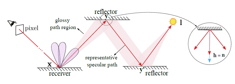
定义
- reflectors:the surfaces that are closer to the light source and are casting caustics
- receiver:the surface that shows the caustics
pathcut 流程
- 问题
- find a representative path for each glossy path region
- compute the radiance distribution, once we have a representative path
3.2 Solution Overview
- 总体思想
- 对于每一个 glossy 的路径区域,找到一条代表性的纯镜面光路(使用 relaxed path cut 算法)
- 使用 SG 积分去近似这条光路上的 radiance 分布,保存在一系列缓存点上(空间复用)
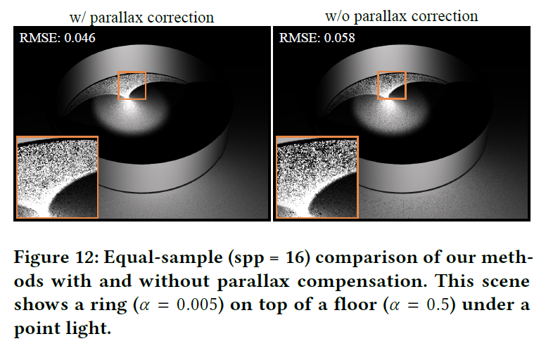
- 渲染的时候,补偿视差,实现精确的 guiding
- 适用范围:caustic
- point light sources and small area light sources
- 只实现了 reflective,(refractive 实现类似)
- constant roughness(不支持 roughness 贴图)
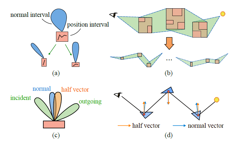
3.3 Relaxed path cuts for glossy materials
搜索阶段
- 我们对区间求交的条件进行一个 relaxed
- 法线区间 \(n\),半角向量区间 \(v\),求他们的点积最大值,如果大于给定值
\(\cos\theta\)
,则认为相交(这条路径可行,可以保留)
- Spherical Gaussian compact-\(\epsilon\) support
\[ \theta=\arccos\left(\dfrac{\ln(\epsilon\pi\alpha^2)\alpha^2}{2}+1\right) \]
- \(\epsilon\) 是阈值,通常设置为 0.01
- \(\alpha\) 表示粗糙程度(roughness)
求解阶段
- 现在我们得到了 leaf path cut
- 使用 Newton solver 进行求解 \(l\)
到 \(x\) 的光路
- 端点 \(l\):光源上的点
- 端点 \(x\):receiver 上的点(焦散显示的点)
一个问题
- 被当作纯镜面的光路求解的时候,求解得到的点可能落在三角形外面,但是对于 glossy 的反射叶来说,仍然和三角形相交
- 此时我们在三角形内部找一个点,使得误差最小
- 找到点之后,我们使用的上面的 SG compact-\(\epsilon\) 公式进行判断是否合理(保留 or 拒绝)
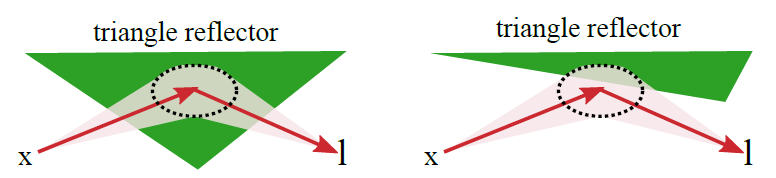
- 此时我们得到了 representative path
讨论
- 当三角形表面法线起伏很大时(bumpy),一个 leaf path cut
可能会有多个解,但是牛顿法只能找到一个解
- Interval Newton 能够找到所有解,但是计算代价很大
- 我们这里直接假设三角形表面的法线起伏小(smooth),因此只存在一个解
- 如果表面材质变得十分粗糙(large roughness),此时 pathcut 的剪枝效率很低,建议用其他方法求解
3.4 Approximating incident illumination with SGs
- 对于上面找到的每一条 representative path,我们需要估计 glossy path region 的贡献
- 之前的方法
- Loubet[Sig20]:slope space
- TO LEARN
- 限制:one intermediate glossy interaction
- Loubet[Sig20]:slope space
- 我们使用基于 SG 的方法,能够扩展到多跳
SG
- Spherical Gaussian(SG)
- \(\mathbf{p}\):中心方向
- \(\lambda\):sharpnes(集中程度)
- \(A\):amplitude(强度)
\[ G(\mathbf{v};\mathbf{p},\lambda,A)=Ae^{\lambda(\mathbf{p}\cdot\mathbf{v})-1} \]
近似 BRDF lobe/slice
- 一个 BRDF lobe 能被一个 SG 近似
- \(\mathbf{p_{\rho}}=2(\mathbf{n}\cdot\mathbf{o})\mathbf{n}-\mathbf{o}\)
- \(\lambda_{\rho}=\dfrac{\lambda_{\text{NDF}}}{4\vert{\mathbf{n}\cdot\mathbf{o}}\vert}\)
- \(C_{\rho}=C_{\text{NDF}}\)
\[ \rho(\mathbf{i},\mathbf{o})\approx G_{\rho}(\mathbf{i};\mathbf{p_{\rho}},\lambda_{\rho},C_{\rho}) \]
- 其中
- \(\mathbf{o}\):view direction
- \(\mathbf{n}\):normal
- \(\lambda_{\text{NDF}}=\dfrac{2}{\alpha^2}\)
- \(C_{\text{NDF}}=\dfrac{1}{\pi\alpha^2}\)
- NDF:normal distribution function
- \(\alpha\):表示材质的粗糙程度
radiance 估计
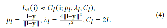
- \(\mathbf{y}\):reflector point
- point light or a small spherical light at position \(\mathbf{l}\) with radius \(r\) and intensity \(I\)
- TO LEARN
SG 乘积
- The product integral of two SGs can be approximated as another SG
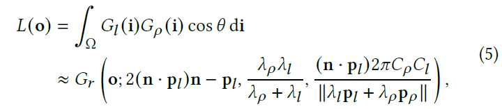
- \(\theta\):\(\langle\mathbf{n},\mathbf{i}\rangle\)
- Since the variation of \(\cos\theta\) over varying \(i\) is subtle, we use \(\mathbf{n}\cdot\mathbf{p}_l\) to approximate it
- 这个式子能够很容易扩展到多个 bounces
shading
- 对于一个着色点(shading point) \(\mathbf{x}\) 来说,来自一个 glossy path region 的入射 radiance 分布被使用一个 SG 来近似
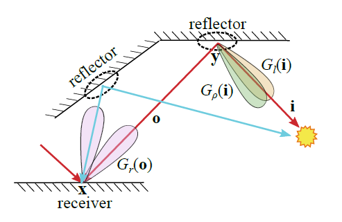
- 如图,上面的结果都是使用 SG 来近似
- \(G_{\rho}(\mathbf{i})\):the radiance at the emitter(SG)
- \(G_{l}(\mathbf{i})\):a BRDF slice with outgoing direction \(\mathbf{o}\)(SG)
- \(G_{r}(\mathbf{o})\):对于每一个
representative specular path,对于从这段 glossy path region 到 \(\mathbf{x}\) 点的入射 radiance 分布被近似为
\(G_{r}(\mathbf{o})\)
- 上面有两个:蓝色、红色
- 使用 GMM 来表示多条 representative specular path 的结果
- GMM:TO LEARN
- 实际过程中发现,相邻的三角形可能会有相同的 reflector
point,因此我们计算不同的 representative paths 上的 reflector
points,如果它们之间的距离小于设定阈值,则认为似乎同一个 reflector point
- 只保留一条 representative path
- 实测发现这样的近似效果很好(更多看补充材料)
3.5 Spatial reusing of representative specular path
- 预计算
- 对每一个着色点都在线运行牛顿法求解是很耗时的
- 观察发现相邻的着色点的入射 radiance 分布类似
- 因此可以离线预计算一部分点(cached points)的入射 radiance 分布(GMMs),然后用这些分布去近似每一个新的 着色点
- shading
- 先找到最近的 cached point 的 GMMs,然后根据视差修正
- 如下图,着色点 \(x\),右边绿色的点是离 \(x\) 最近的 cached point \(y\)
- 此时橙色的是 \(y\) 的入射 radiance 分布 SG1,紫色的是应该近似成的入射 radiance 分布 SG2
- 此时我们将 SG1 进行旋转,实现由于视差导致的补偿
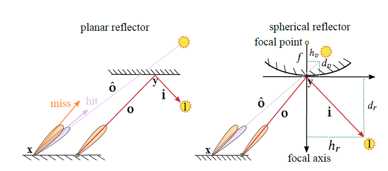
- 如何旋转?
- 计算 emitter 关于 reflector 的像,然后把镜像和着色点 \(x\) 连线,计算得到正确的方向 \(\hat{\mathbf{o}}\)
- 这里的 reflector 指的是 representative specular path 中到达 cached point 之前的最后一个 reflector
- 将 SG1 的中心方向 \(\mathbf{o}\) 旋转为 \(\hat{\mathbf{o}}\)
- 计算 emitter 关于 reflector 的像,然后把镜像和着色点 \(x\) 连线,计算得到正确的方向 \(\hat{\mathbf{o}}\)
如何旋转
- Ruppert et al. 2020
- the parallax-aware representation for planar reflection
- TO LEARN
- 受这个启发,我们通过将曲面拆分为两个具有不同主方向(principal directions)的 reflectors,从而能够纠正任意曲线的 reflector 的视差
Spherical reflector
- 示意图如上图的右子图
- 两个主轴
- the focal axis(normal)
- the sphere’s tangent axis(tangent)
- 计算像点(凸面镜成像公式)
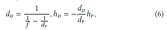
- focal length \(f\)
- concave mirror(凹面镜):positive
- convex mirror(凸面镜):negative
- 计算得到像点之后,连接得到修正的 SG 的主方向 \(\hat{\mathbf{o}}\)
Arbitrary-curved reflector
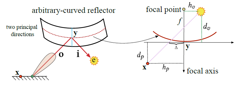
- 对于任意曲面的 reflector 来说,不存在视角无关的像的位置
- 对于任意曲面,可以找到两个主曲率方向(principal curvature directions),可以把这个曲面使用 focal axis 为主曲率方向的两个 spherical reflector 来近似
- 对于每一个方向求解一个像点
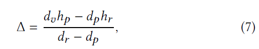
- 这个时候我们会得到一个偏移量(上图中的 \(\Delta\) )
- 对两个方向的偏移量进行叠加,得到总的偏移量,总的偏移量定位了像的位置
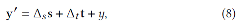
- \(\mathbf{s},\mathbf{t}\) 是两个主曲率方向,两个 \(\Delta\) 对应各自的偏移量
- 修正的 SG 的方向为 \(\mathbf{xy'}\)
- 这样的视差补偿只适用于 one-bounce
的反射,对于 multi-bounces 的情况,我们将之前的
reflector 都当作 spherical reflector
- 具体的见补充资料
讨论
- 缓存点的建立
- 我们的三角形大小都是相似的,为每一个 receiver 上的三角形生成一个缓存点,然后构建一个 pont cloud
- 如果三角形的大小是任意的,建议在三角形内部采样
- 缓存点数据
- GMM
- 用于视差补偿的信息
- \(d_v,h_v\)
- reflector point \(\mathbf{y}\)
- tangent frame at \(\mathbf{y}\)
3.6 Rendering
- 相机发射光线,光线和某个三角形相交
- 找到这个三角形上关联的缓存点,得到 GMM
- 对 GMM 内部的所有 SG 进行视差补偿,构建新的 GMM
- 使用 MIS 对 BRDF 采样和对 GMM 联合采样,采样一个出射方向,递归进行
- constant probability(0.5)
- 对每一个 bounce 都使用 NEE(next event estimation)
讨论
- 我们对每一个 GMM 添加了一个保护性的 smooth lobe(覆盖整个半球),这样保证所有可能方向都被采样到
- 无偏的(证明作为后续工作)
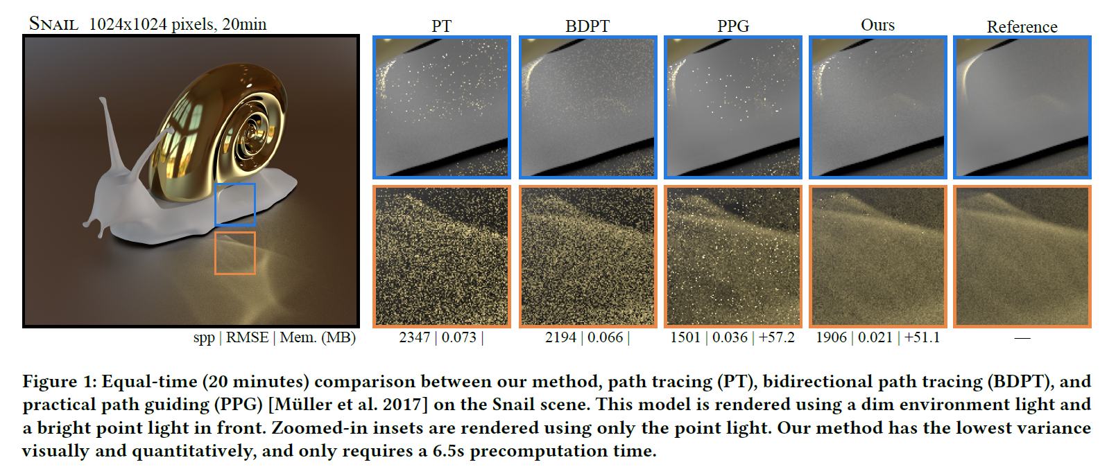
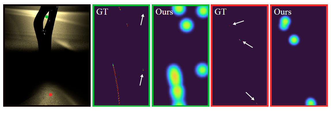
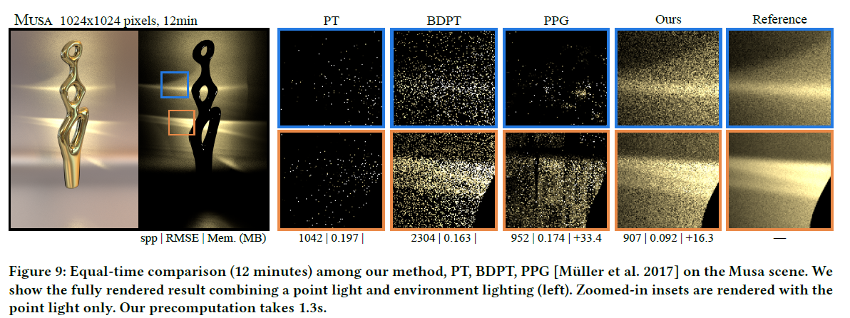
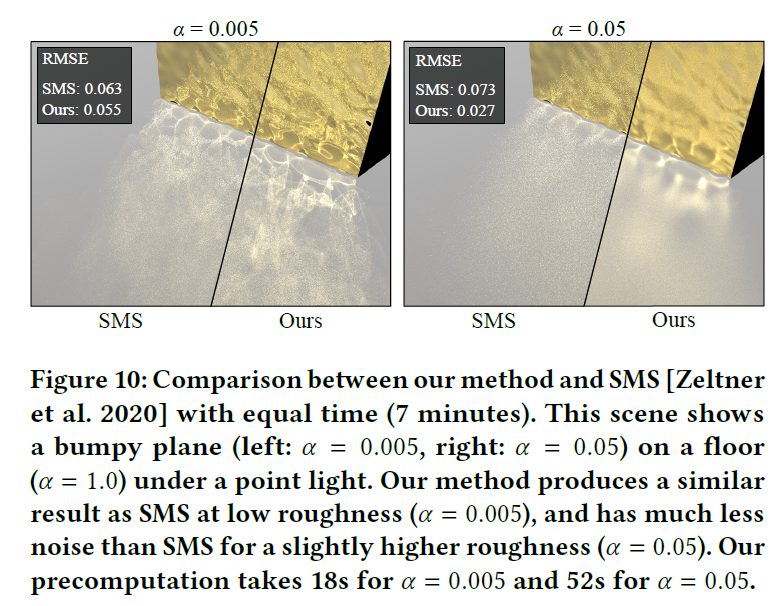
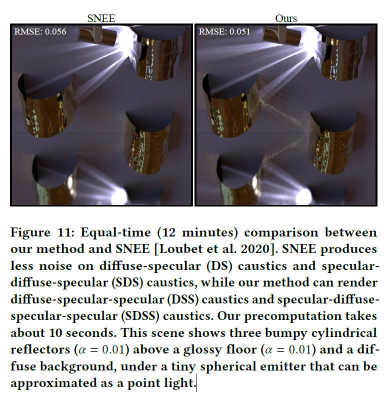
4 RESULTS
- 利用 mitsuba 实现
- 支持材质:rough conductor as reflector olny
- 对比算法
- PT、BDPT、PPG、SMS(specular manifold sampling)、SNEE(specular next event estimation)
- reference:65536spp with BDPT
- equal time
- the precomputation and the rendering
- 测试环境
- 4.20GHz Intel i7 (8 cores) with 16 GB of main memory
- RMSE(Root Mean Square Error)
- 我们的算法支持
- point light
- small sphere lights with less than 0.01 radian (radius/distance)
- 环境光留给 PT
- 场景设置
- 突出 one-bounce or multi-bounce reflective caustics
5 DISCUSSION AND LIMITATIONS
对比其他方法
视差校准
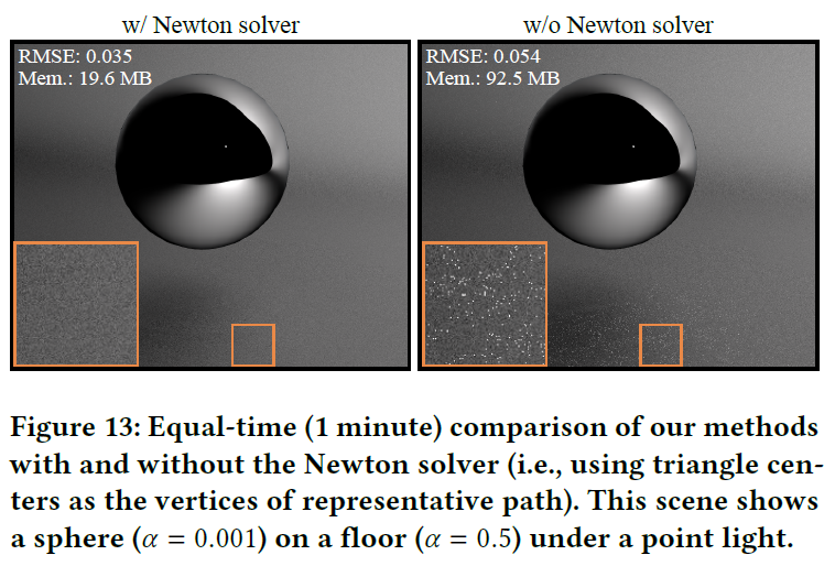
牛顿法求解
- 不使用牛顿法求解,则直接使用三角形中心来表示 representative specular path 中的节点
6 CONCLUSION
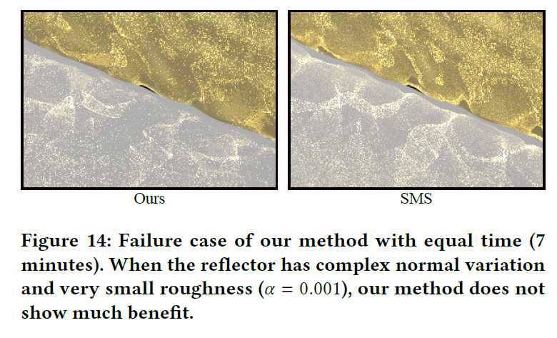
limitation
- Performance:跳数多跑得慢
- 我们的实现最多支持两跳
- small roughness 效果好
- Extremely low-roughness materials:SG 近似和视差修正不够准确
- Subdivision of the meshes:网格需要足够细分,才能够有效找到路径
- densely tessellated