(论文)[2018] Geometry-Aware Metropolis Light Transport

Posted on 2022-02-08 Edited on 2022-02-21 In CG.Paper Views:

MLT 对 path segment 的出射角度进行变异的时候，利用可见性求出没有遮挡的最大圆锥，将变异的最大角度设置为圆锥顶角，从而避免因为可见性原因导致新生成的路径被拒绝

GeoMLT

Geometry-Aware Metropolis Light Transport
Hisanari Otsu, Johannes Hanika, Toshiya Hachisuka, and Carsten Dachsbacher. 2018. Geometry-Aware Metropolis Light Transport. ACM Trans. Graph. 37, 6, Article 278 (November 2018), 11 pages. https://doi.org/10.1145/3272127.3275106

0. 展示

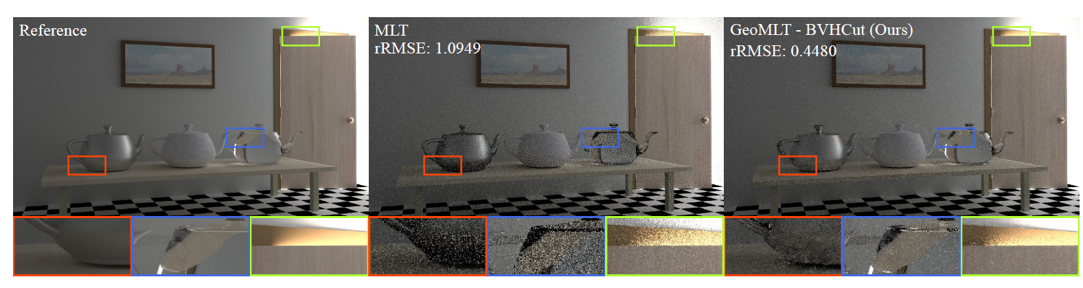
30 分钟渲染的结果，光源在门外
- reference 是通过 BDPT 渲染收敛得到
传统的 MLT 在边界、间隙的时候由于可见性的改变，变异得到的路径常常会被拒绝，我们的方法根据几何信息控制变异的大小
- adaptively controls the mutation size according to the geometry information surrounding each path segment
我们的方法能够很好的避免由于可见性导致的零贡献样本（不可见）
通过估计最大的可见的圆锥顶角来限制突变步长，从而避免可见性问题
- 在不降低采样质量的前提下，提高 MLT 突变的接受率
直接估计代价较大，我们还提出了加速方式

1. INTRODUCTION

MCMC 渲染方式
高效的 MCMC 取决于如下因素
- the design of the transition kernel (path mutation)
  - 小步长的样本 \(\to\) 和之前的样本比较像 \(\to\) 较高的接受率
- the autocorrelation between states
  - 自相关程度高 \(\to\) 样本附加信息少 \(\to\) 样本质量低
  - 步长大 \(\to\) 容易被拒绝
通过局部结构来控制变化的步长
我们着重考虑因为可见性问题（不可见）导致的被拒绝的路径
如下图，蓝色范围表示突变核 kernel
- 右边的 kernel 更好，左边可能会产生由于不可见而被拒绝的路径，右边不会

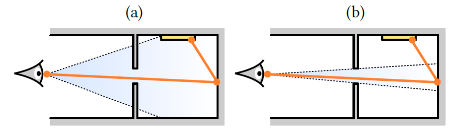
现在的考虑可适应步长的方法没有考虑可见性问题
- Wenzel Jakob and Stephen Marschner. 2012. Manifold exploration: a Markov chain Monte Carlo technique for rendering scenes with difficult specular transport. ACM Transactions on Graphics (Proc. SIGGRAPH) 31, 4, Article 58 (2012).
- Tzu-Mao Li, Jaakko Lehtinen, Ravi Ramamoorthi, Wenzel Jakob, and Frédo Durand. 2015. Anisotropic Gaussian Mutations for Metropolis Light Transport Through Hessian-Hamiltonian Dynamics. ACM Transactions on Graphics (Proc. SIGGRAPH Asia) 34, 6 (2015), 209:1–209:13.
我们第一次在 MCMC 中考虑了可见性因素
文章的贡献
- 第一次在 MCMC 中考虑了可见性因素
- 如上图所示，给出了一种快速估计最大的圆锥顶角的算法
- 很容易集成到现有的 MLT 算法中，我们给出了实现

2. BACKGROUND AND PREVIOUS WORK

2.1 Light Transport Simulation

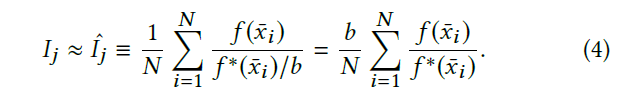
intensity \(I_j\) of the \(j\)-th pixel
- 论文中之后把 \(f_j\) 简写为 \(f\)

\[ I_j=\int_{\Omega}f_j(\bar{x})\;\mathrm{d}\mu(\bar{x}) \]

\(\Omega\)：任意长度、所有可能的路径空间

\[ \Omega=\bigcup_{k=2}^{\infty}\Omega_{k} \]

\(\Omega_{k}\)：结点数为 \(k\) 的路径空间
\(\bar{x}\)：路径
- \(\bar{x}=(\mathrm{x}_1,\cdots,\mathrm{x}_k)\in\Omega\)
\(\mathcal{M}\)：场景表面集合
- \(\mathrm{x}_i\in\mathcal{M},\;i=1,\cdots,k\)
采样算法
- Path Tracing：Kajiya 1986
- Light Tracing：Arvo 1986
- BDPT：Lafortune and Willems 1993; Veach and Guibas 1994

2.2 MCMC Rendering

论文这一段是对 MLT 的介绍
MCMC：MLT
- Veach and Guibas 1997
- 把 \(f\) 作为目标分布的时候，最终路径的分布会趋近于 \(f/b\)（归一化后的分布）
\[ b=\int_{\Omega}f(\bar{x})\;\mathrm{d}\mu(\bar{x}) \]
Metropolis-Hastings (MH) algorithm
- Hastings 1970; Metropolis et al. 1953

算法

生成一系列的路径样本，新样本 \(y\) 的生成只依赖于上一个样本 \(x\)，转移核 \(T\)

\[ \bar{y}\sim T(\bar{x}\to\bar{y}) \]

新样本以一定概率被接受

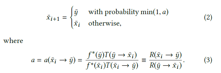
最后一部分等式推导

\[ R(\bar{x}_i\to\bar{y})\equiv f (\bar{y})/T(\bar{x}_i\to\bar{y}) \]

\(f^{\ast}\)：the scalar contribution function, which typically is the luminance of \(f\)

变异策略

变异策略基于状态空间
- PSSMLT：Kelemen et al. [2002]
- MMLT：Hachisuka et al. [2014]
  - 利用 MIS 将 PSSMLT 和 BDPT 结合在一起
- Three recent works by Pantaleoni [2017], Otsu et al. [2017], and Bitterli et al. [2017] concurrently proposed techniques to combine the different state spaces by using an inverse mapping from the primary sample space to the path space.

2.3 Path Space Perturbations

Our geometry-aware mutation technique is based on the lens, caustic, and multi-chain perturbations operating in the path space [Veach and Guibas 1997].
对于一条 subpath，我们对其的扰动为改变它的出射方向（局部球面坐标系）
- 例如扰动从 lens 出发的 subpath，我们改变其出射方向，追踪这条光线，直到停在 diffuse 的表面

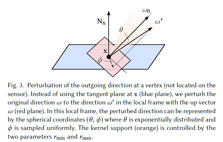
以出射方向为上方向，\(\theta\) 指数分布，\(\phi\) 均匀分布
- Veach and Guibas [1997]

采样得到的 \(\theta\in[r_{\min},r_{\max}]\)
\(U\)：\([0,1]\) 均匀分布
推导得到 pdf 如下

如何设置步长（也就是设置 \(r_{\max},r_{\min}\)）对于渲染结果影响很大
- 自相关性 vs 收敛速度

2.4 Adaptive Step Sizes

有些研究根据目标函数的某些特征实现可适应步长
- Li et al. [2015] utilized local information obtained from analytic derivatives to adaptively control the shape of the transition kernels based the idea of Hamiltonian Monte Carlo [Duane et al. 1987].
- Jakob and Marschner [2012]
  - specular 表面，将路径空间限制在低维度中
- Kaplanyan et al. [2014] and Hanika et al. [2015]
  - 泛化上面的方法，使用半角向量表示路径空间
之前的方法都没有考虑可见性的问题，因为可见性函数的微分包含狄拉克函数成分 \(Dirac\)

2.5 Cones in Rendering

Cone tracing [Amanatides 1984]
- 使用 cone 代替了 ray 和场景求交
- 有效的实现了 AA
Roger et al. [2007]
- 使用 cone 表示一组 ray，从而实现了一组相关的光线和场景的快速求交
  - 可能有用
Mora [2011]
- utilized cones as ray packets in the context of divide-and-conquer ray tracing.
Crassin et al. [2011]
- voxelized scene geometries
我们在一条出射光线的周围放置一个 cone，找到最大的不和场景相交的 cone

3 OVERVIEW

3 个问题
- 如何找到最大的张角？
- 如何加速？
- 如何集成到 MLT 中？

例子

引导性的例子 MLT vs GeoMLT（场景与测试结果）

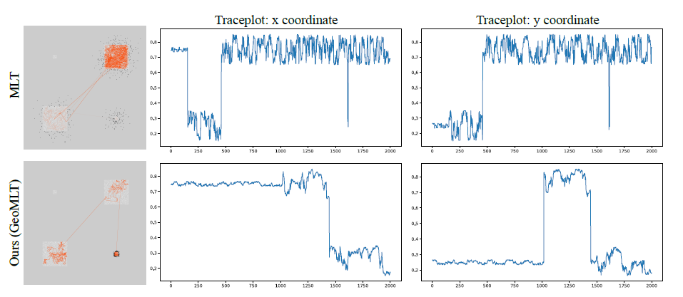
如上，黑点表示被拒绝的样本，橙点表示接受的样本
限制路径长度为 1，被拒绝的原因只有可见性
上面的图示表示 GeoMLT 的适应性步长有比较好的效果

4 GEOMETRY-AWARE PERTURBATION SIZE

让变异范围内的光线都不会因为可见性原因而被拒绝
如何计算 cone 的最大张角 \(r_{\max}\)
- 通过用户定义的一个参数 \(\alpha\) 求得 \(r_{\min}=\alpha r_{\max}\)
path segment：\(\mathrm{x}_1\mathrm{x}_2\)
点 \(\mathrm{x}_1\) 不动，扰动出射方向

truncated cone

引入 truncated cone 的概念

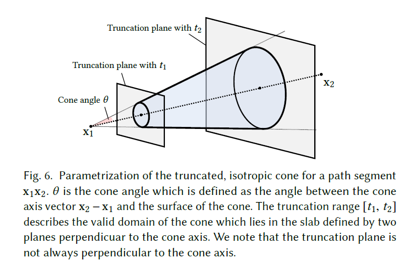
两个截断平面
- 避免自相交、和点 \(\mathrm{x}_2\) 比较近的几何体的相交
- The truncation of the cone’s apex and the base is used to avoid self-intersections close to \(\mathrm{x}_1\) and to avoid unnecessary small cone angles due to geometry close to \(\mathrm{x}_2\)

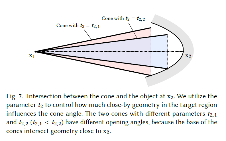
\(t_2\) 截断平面不一定和圆锥的轴垂直
- 更好的考虑倾斜的几何体
- 使用交点 \(\mathrm{x}_2\) 的法线作为平面的法线
\(t_1\) 需要垂直
\(\mathcal{C}(\theta)\)：所有在上面的 truncated cone 之间的点的集合
场景表面集合：\(\mathcal{M}\)
则最大的张角如下

\[ \theta_{\max}=\sup\{\theta\vert\mathcal{M}\cap\mathcal{C}(\theta)=\emptyset\} \]

准确计算十分耗时
- 一种方法是二分的进行 cone-scene intersection test

5. APPROXIMATE CONE ANGLE

粗略估计
使用 AABB 包围盒代替几何体进行 \(\theta_{\max}\) 的计算

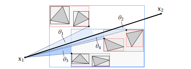
5.1 Estimating the Cone Angle for a Single AABB

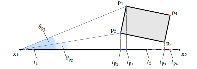
计算一个 path segment 和一个 AABB 的 \(\theta_{\max}\)
求出相交的最小夹角，算法如下
- 如果某个顶点 \(\mathrm{p}_i\) 在 \([t_1,t_2]\) 之间，计算夹角 \(\langle \mathrm{x}_1\mathrm{p}_i,\mathrm{x}_1\mathrm{x}_2\rangle\)
- 对于 AABB 的每一条边，我们求出到 \(\mathrm{x}_1\mathrm{x}_2\) 最近的点，如果这个点落在 \([t_1,t_2]\) 之间，用它更新夹角
- \(t_2\) 平面和 AABB 求交（得到一个凸多边形），求这个凸多边形到 \(\mathrm{x}_1\mathrm{x}_2\) 最近的点，更新夹角
如下图
- \(\mathrm{p}_1,\mathrm{p}_2\) 的投影在区间 \([t_1,t_2]\) 内部，需要考虑
- \(\mathrm{p}_3,\mathrm{p}_4\) 的投影在区间 \([t_1,t_2]\) 外部，不需要考虑

5.2 Cone Estimation using a BVH-Cut

首先计算 initial cut，里面包含如下的结点
- 他们的父结点和 \(\mathrm{x}_1\mathrm{x}_2\) 相交，但是他自己没有和 \(\mathrm{x}_1\mathrm{x}_2\) 相交
- 如下的红色结点

实现如下

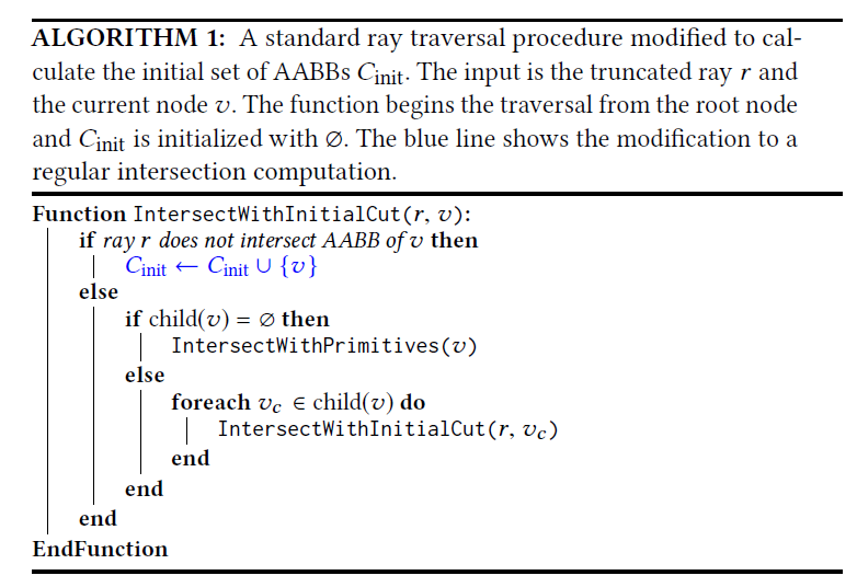
此时 initial cut 里面包含着一堆绕着 \(\mathrm{x}_1\mathrm{x}_2\) 的 AABB，但是他们都不和 \(\mathrm{x}_1\mathrm{x}_2\) 相交
这也可以避免角度变成 0（和空的 AABB 相交）
- 会被排除
此时可以使用 5.1 的方法对每一个 AABB 进行求解
- 如此得到的 \(\theta_{\max}\) 总是会偏小

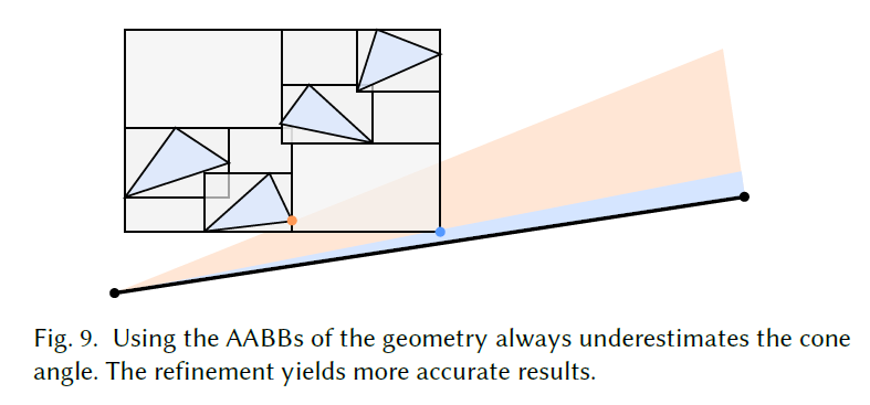
优化策略：将所有的 AABB 展开，直到结点个数达到设定值 \(N_{\max}\)
- 优先队列 \(Q\)，夹角最小的在根结点

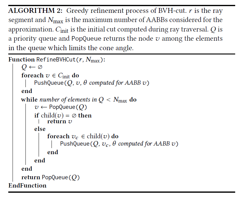
展开每个结点，直到限制夹角的结点为叶子结点（此时已经是最大）或者达到数量限制（考虑效率）

5.3 Trading Accuracy for Speed

更快但是牺牲了准确率
一种策略：只进行 5.1 部分的第一个测试（顶点），而且不进行 cut refinement

6. GEOMETRY-AWARE METROPOLIS LIGHT TRANSPORT

扰动策略
- a geometry-aware extension of the multi-chain perturbation
可以类似的迁移到其他的扰动策略上
- lens or caustic perturbation

变异策略

当前路径：\(\bar{x}=\mathrm{x}_1\mathrm{x}_2\cdots\mathrm{x}_k\)
依次对这样的 path segment 进行扰动，直到遇见两个连续的非镜面顶点
- \(\mathrm{x}_i\mathrm{x}_{i+1}\)：出发自非镜面，终止在镜面
- 突变从 \(\mathrm{x}_k\) （光圈）开始，突变策略就是上面讲的
- 保证结点的表面类型、结点数量不变
- 结果为 \(\bar{y}=\mathrm{x}_1\mathrm{x}_2\cdots\mathrm{x}_s\mathrm{y}_{s+1}\cdots\mathrm{y}_k\)
优化
- 如果 \(\mathrm{x}_{i+1}\) 是非镜面或者光圈，我们扰动原始的方向（\(\omega_0=\mathrm{x}_{i+1}\to\mathrm{x}_i\)），此时下一个顶点 \(\mathrm{y}_i\) 通过朝着新的方向 \(\omega\) 射出一条光线计算得到，不使用方向 \(\mathrm{y}_{i+1}\to\mathrm{x}_i\)，因为这样在计算接受率的时候需要额外对这段路径进行可见性测试
- 如果 \(\mathrm{x}_{i+1}\) 是镜面，则根据确定的方向计算得到 \(\mathrm{y}_i\)

计算接收率

化简，消去公共项（前面一段相同）

只需要计算不同的项

7. RESULTS

MLT：\(r_{\max}=0.5,r_{\min}=0.05\)
GeoMLT：\(N_{\max}=10,\alpha=0.1\)
算法
- the bidirectional mutation for global exploration
- and the multi-chain perturbations for local exploration with equal selection probability.

实现

Clamping the Estimated Cone Angle
- 如果光线掠过一个几何体的表面，可能会导致计算得到的 \(\theta\) 很小（几乎为 0），我们将计算得到的 \(\theta\) clamp 到用户指定的范围内
- 实验为 \([0.01,0.5]\)
Avoiding Unnecessary Cone Angle Underestimation
- \(t_2\) 设置得距离 \(\mathrm{x}_2\) 不能太近
- 实验：\(t_1=10^{-4},t_2=0.99\Vert\mathrm{x}_1-\mathrm{x_2}\Vert\)
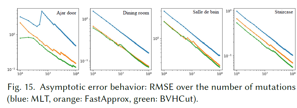
Equal-Time Comparisons
- 我们的方法不对出发于镜面的顶点进行估计，因此在这种情况下会有问题
Accuracy of the BVHCut Approximation
- BVHcut 估计的顶角范围基本准确
- 算法能够适应不同场景（场景旋转不同角度，AABB 改变）
Quality of Exploration
- 评估：\(\text{MCMC-SE}=\sqrt{\dfrac{\text{Var}}{\text{ESS}}}\)

Differently-Sized Geometry
- 场景中同时有不同尺度的几何体
- 树干和树枝
- 背景中含有一个很大的 diffuse reflector 时，我们看到 GeoMLT 增益不大
  - 因为可以跳过这个遮挡的树枝，从另外的一个间隙中过来，因此 \(\theta\) 之外其实也还有很多可行的光路

8. DISCUSSION

Parameters
- 有些人为设置的参数，会影响渲染结果
Cone Angle Estimation
- BVHCut：相对精确
- FastApprox：很宽松
- 更好的方法：TODO
Limitations
- 两个顶点都是镜面材质
- 不连续结构
- 最大张角很大（大于等于人为设置的最大值），此时 BVHCut 白做了
Reusing Acceleration Structure
- 同时进行，方便
Future work
- 各向异性的 cone
- 现在只支持表面渲染，推广到参与介质的渲染（participating media）
- designing geometry-aware mutations in primary sample space

9. CONCLUSION

We presented a mutation strategy which adaptively changes the mutation step size according to the geometry of the scene. Our method restricts perturbations of path segments such that nearby geometry is not intersected, as this would always result in rejected proposals. We introduced fast, approximate algorithms to estimate the maximum perturbation angle, which reuse the very same acceleration structure which is already present for ray casting.We demonstrated that our approach can greatly improve the exploration performance of a Markov chain. Our perturbation strategy has been designed with small geometric features in mind, such as door slits or keyholes where the light shines through. However, as our results show, it also reduces noise near geometric edges, such as the one between the floor and the back wall in the Ajar door scene. We believe that using information about geometric visibility has great potential and can be used to ameliorate many other cases of inefficient mutations due to geometric constraints.