(论文)[2012] Light Transport Simulation with Vertex Connection and Merging
Light Transport Simulation with Vertex Connection and Merging
SIGGRAPH Asia 2012
效果展示
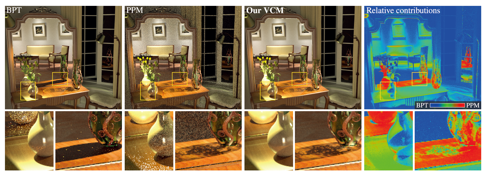
- BPT(Bidirectional Path Tracing)
- 不能很好的模拟 caustics 现象
- 例如 SDS 路径
- PPM(Stochastic Progressive Photon Mapping)
- PPM has difficulties in handling the illumination coming from the room seen in the mirror
- TODO
- VCM = BPT + PPM
- 通过多重重要性采样的方法将这两种方法结合起来
- MIS(Multiple Importance Sampling)
- 文章代码
1. Introduction
- 之前的方法基本存在的问题,不能在所有场景中都发挥得很好
- 在某些场景中不能表现得很好
- 忽略某些类型的光路
BPT
- 能够处理大部分场景
- MIS 的采样方法能够很好的将很多种光路组合起来
- The true key to its robustness is the provably good combination of various path sampling techniques using MIS.
- 不好处理 SDS 的光路
- ‘specular’ also includes sharp glossy interactions
- 原因是这样的光路被采样的概率很小,尤其是 point light sources + pinhole cameras 场景的时候
PM
- 能够很好地处理 SDS 光路
- Its inefficiency under diffuse lighting and its relatively low order of convergence
- 存在的问题
- 收敛很慢
- 在 diffuse lighting 条件下,效果不太好
BPT + PM
- 之前有人将 BPT 和 PM 结合过,但是效果不太好
- Combining BPT with PM via heuristic classification of paths into caustic and non-caustic can be far from optimal
- 启发式的将路径分为焦散路径和其他路径
- 我们使用 MIS 的技术将 BPT 和 PM 结合
- 之前大家把 BPT 和 PM 放置在两套数学框架下,下载我们提出新的思路,从而将这两个方法结合起来
- 通过 MIS 结合起来的方法能够很好的保留二者的优点
- 保有 BPT 的 MSE 收敛率 \(O(\dfrac{1}{N})\)
- 保有 PM 对于 SDS 路径的高效查找
论文的贡献
- A novel reformulation of photon mapping compatible with the path
integral formulation of light transport (Section 4)
- 重新定义了 PM 算法的数学框架,使其和路径积分兼容
- A robust light transport simulation algorithm that combines BPT and
PM via multiple importance sampling (Section 5)
- 一个结合了 BRT/PM 长处的算法
- A progressive variant of the combined algorithm along with an
asymptotic analysis of its error convergence (Section 6)
- 方差的渐进分析
2. Previous Work
Path tracing
- 从相机出发
- [Kajiya 1986]
- 从光源出发
- Dutr´e et al. [1993]
- 双向:BPT
- [Lafortune and Willems 1993; Veach and Guibas 1994]
- path integral framework
- PT 的积分框架
- Veach [1997]
- MIS,多条采样路径
- [Veach and Guibas 1995]
Photon mapping
- 有偏的
- density estimation:光子密度估计
- [Jensen 2001]
- photon mapping has difficulties in scenes with
many glossy objects
- Haˇsan et al. [2009] and Vorba [2011]
- 利用 MIS,组合多条 eye sub-path
- Vorba [2011]
- 对于 PM 的定义不能很好的利用 MIS 将 PM 和 BPT 结合
- MIS,让 PM 在 glossy 材质上的焦散表现得更好
- Tokuyushi [2009]
- PPM
- [Hachisuka et al. 2008]
- 因为 PM 是有偏的,PPM 通过减小半径的方式,试图减小 bias
- 相较于 BPT,更好的模拟 SDS 光路,但是渐进误差收敛速率更慢
- asymptotic error convergence rate
- Hachisuka et al. [2010] 给出估计
Markov chain Monte Carlo
- MCMC
- MCMC 能够更多的采样具有贡献的 path(让我们接受的 path)
- BPT [Veach and Guibas 1997]
- PM/PPM [Fan et al. 2005;Hachisuka and Jensen 2011]
Many-light methods
- [Keller 1997; Walter et al. 2006; Haˇsan et al. 2007; Ou and Pellacini 2011]
- [Kˇriv´anek et al. 2010]
- 能量损失、失真问题
- [Kollig and Keller 2004; Haˇsan et al. 2009; Davidoviˇc et al. 2010;
Walter et al. 2012]
- 减轻上面的问题
- 都不能很好的处理 SDS 光路
3. Background
MIS
- Multiple importance sampling
- [Veach and Guibas 1995]
- 我们要求积分 \(I\),其中\(f(x)\) 为实值函数,\(\mu(x)\) 是积分域 \(\Omega\) 上的测度
\[ I=\int_{\Omega}f(x)\;\mathrm{d}\mu(x) \]
- MIS 构造了一个对 \(I\)
的无偏估计,这个无偏估计是通过组合 \(m\)
个不同的分布(采样方法)得到的组合估计,每一种分布以 \(p_i\) 给出它的 \(\mathrm{pdf}\)
- \(X_{i,j}\) 为满足分布 \(p_i\) 的随机变量
\[ \langle I\rangle_{MIS}=\sum_{i=1}^m\dfrac{1}{n_i}\sum_{j=1}^{n_i}w_i(X_{i,j})\dfrac{f(X_{i,j})}{p_i(X_{i,j})} \]
- 最小化估计的方差,权重设置
\[ w_i(x)=\dfrac{\left[n_ip_i(x)\right]^\beta}{\sum_{k=1}^n\left[n_kp_k(x)\right]^\beta} \]
- \(\beta=1\)
- 具体分析看论文:TODO
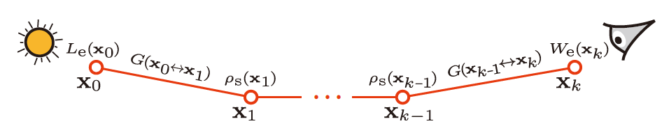
Path Integral Framework
- [Veach 1997]
- 积分框架
\[ I=\int_{\Omega}f(\bar{\mathrm{x}})\;\mathrm{d}\mu(\bar{\mathrm{x}}) \]
- \(\bar{\mathrm{x}}\) 表示一条可行的光路,\(\bar{\mathrm{x}}=\mathrm{x}_0\cdots \mathrm{x}_k\),其中有 \(k(k>0)\) 条边,\(k-1\) 个中间结点
- \(\mathrm{x}_0\) 在光源处,\(\mathrm{x}_k\) 在摄像机上
- \(\Omega\) 表示任意长度的光路
- 面积测度:\(\mathrm{d}\mu(\bar{x})=\mathrm{d}A(x_0)\cdots\mathrm{d}A(x_k)\)
- 贡献测度:\(f(\mathrm{\bar{x}})\)
\[ f(\bar{\mathrm{x}})=L_e(\mathrm{x}_0){\color{red}G(\mathrm{x}_0\leftrightarrow\mathrm{x}_1)\left[\prod_{i=1}^{k-1}\rho_{s}(\mathrm{x}_i)G(\mathrm{x}_i\leftrightarrow\mathrm{x}_{i+1})\right]}W_e(\mathrm{x}_k) \]
- 红色部分记作 \(T(\mathrm{\bar{x}})\;{\buildrel\rm def\over=}\;\mathrm{path\ throughput}\)
- \(L_e(\mathrm{x}_0) = L_e(\mathrm{x}_0\to\mathrm{x}_1)\) 表示光源从 \(\mathrm{x}_0\) 向 \(\mathrm{x}_1\) 发射的 radiance
- \(W_e(\mathrm{x}_k) = W_e(\mathrm{x}_{k-1}\to\mathrm{x}_k)\) 表示摄像机在 \(\mathrm{x}_{k}\) 点,对从 \(\mathrm{x}_{k-1}\) 点入射到 \(\mathrm{x}_{k}\) 的光的灵敏性
- \(\rho_{s}(\mathrm{x}_i)=\rho_{s}(\mathrm{x}_{i-1}\to\mathrm{x}_i\to\mathrm{x}_{i+1})\):在 \(\mathrm{x}_i\) 点的 BSDF
- \(G(\mathrm{x}_i\to\mathrm{x}_j)=V(\mathrm{x}_i\to\mathrm{x}_j)\dfrac{\vert\cos\theta_{i,j}\vert\vert\cos\theta_{j,i}\vert}{\Vert\mathrm{x}_i-\mathrm{x}_j\Vert^2}\):表示几何项
- \(V\) 表示几何项
- 简单的可以把 \(f(\bar{\mathrm{x}})\) 记作
\[ f(\bar{\mathrm{x}})=L_e(\mathrm{x}_0)T(\bar{\mathrm{x}})W_e(\mathrm{x}_k) \]
- 上面的表达式能够让 MIS 方法生效
\[ \dfrac{f(\bar{\mathrm{x}})}{p(\bar{\mathrm{x}})} \]
Path sampling techniques
- \(p(\bar{\mathrm{x}})\) 是联合分布
- 每一步的采样都是独立的
\[ p(\bar{\mathrm{x}})=p(\mathrm{x}_0,\cdots,\mathrm{x}_k)=p(\mathrm{x}_0)\cdots p(\mathrm{x}_k) \]
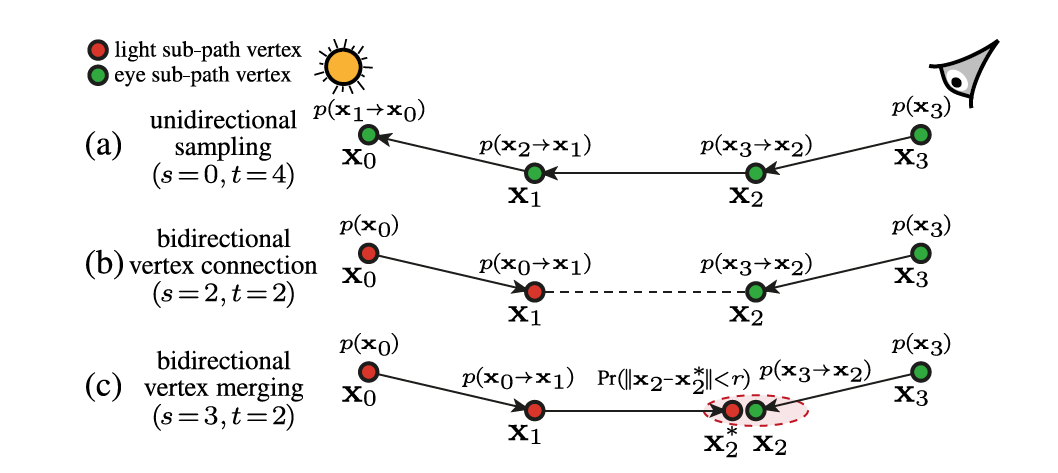
- \(p(\mathrm{x}_j)\) :方向采样的概率
\[ p(\mathrm{x}_j)= \left\{ \begin{array}{**lr**} p(\mathrm{x}_{j-1}\to\mathrm{x}_{j}), & \mathrm{if\ x_{j}\ is\ on\ a\ light\ subpath} \\ p(\mathrm{x}_{j}\to\mathrm{x}_{j-1}), & \mathrm{if\ x_{j}\ is\ on\ a\ eye\ subpath} \\ \end{array} \right. \]
- BPT 中一条长度为 \(k\) 段的光路的产生可以有 \(k+2\) 种方式
- BPT 最早的实现
- [Lafortune and Willems 1993; Veach and Guibas 1994]
- MIS,组合不同的采样路径,同时使用指数的形式
- 因为如果不加指数,会把出现概率很小的 SDS 路径直接剪掉
- 按照上面的采样方法,对于 SDS 路径只有两种方式(单项路径),而这样的光路采样概率很小,导致方差很大
- MIS automatically diminishes the weight of a sampling technique that is inappropriate (i.e. has a low pdf value) for a given path
- [Veach and Guibas 1995]
- 因为如果不加指数,会把出现概率很小的 SDS 路径直接剪掉
Photon mapping radiance estimate
- [Jensen 2001]
\[ L_s(\mathrm{x},\omega)\approx\sum_jK_r(\Vert\mathrm{x}-\mathrm{x}_j\Vert)\rho_{s}(\omega_j,\mathrm{x},\omega)\Phi_j \]
- \(K_r\):2D 滤波核,半径 \(r\)
- \(j\):到 \(\mathrm{x}\) 的距离小于 \(r\) 的所有光子
- \(\omega_j\):光子的入射方向
- \(\mathrm{x}_j\):光子的位置
- \(\Phi_j\):光子的光通量 flux
- \(\omega\):eye ray 的入射方向
- \(\rho_s\):BSDF
- 这样看来,PM 和 BPT 并不是定义在一套数学框架下的,PM 甚至与采样的路径无关,因此很难用 MIS 将他们结合起来
4. Vertex Merging
- 首先我们需要将 PM 和 BPT 用一个数学框架描述
- 将 PM 用积分框架进行描述
- 我们接下来的讨论把 light path 长度规定为 \(k\)
- PM radiance 的估计可以发生在第 \(s\) 个结点上
- 这样就产生了单路径采样的方法
- 整套方法需要通过估计光路上的不同 \(s\) 的值,\(s\in[1,\cdots,k-1]\)
PM as a sampling technique for extended paths
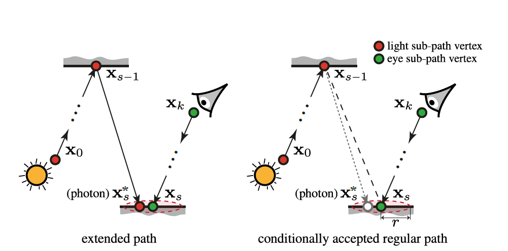
- 把 PM 的光路当作单路径采样得到的结果
- 自然的想法,我们对一个光子产生的光路,只考虑光子在最终的位置 \(\mathrm{x}_s^\ast\)
- 整条路径为 \(\mathrm{x}_0,\cdots,\mathrm{x}_s^\ast\)
- 我们用于做密度估计的点 \(\mathrm{x}_s\) 需要是一条从摄像机出发的 sub-path \(\mathrm{s}_0,\cdots,\mathrm{x}_k\)
- 这样最终组成一条路径 \(\mathrm{x}_0,\cdots,\mathrm{x}_s^\ast,\mathrm{x}_s,\cdots,\mathrm{x}_k\)
- 记作
extended path,\(\bar{\mathrm{x}}^\ast=(\mathrm{x}_0,\cdots,\mathrm{x}_s^\ast,\mathrm{x}_s,\cdots,\mathrm{x}_k)\) - 上面的左图
- 记作
- 整条路径的概率
\[ p(\bar{\mathrm{x}}^\ast)=p(\mathrm{x}_0,\cdots,\mathrm{x}_s^\ast)p(\mathrm{x}_s,\cdots,\mathrm{x}_k)=p(\mathrm{x}_0)\cdots p(\mathrm{x}_s^\ast)p(\mathrm{x}_s)\cdots p(\mathrm{x}_k) \]
Discussion
- 我们现在已经把 PM 当作是一种采样策略,生成一条extended
path,同时它有自己的 pdf
- extended path 比正常的 path(BPT)多出一个点 \(\mathrm{x}_s^\ast\) (光子的位置)
- pdf 更高维,于是在权重估计上会出问题
- 为了能够使用 MIS 将 BPT 和 PM 结合起来,需要将二者的长度修改为一致
- 两种都可以,这里采用 BPT 的长度(可以保证原来的积分形式不变)
PM as a sampling technique for regular paths
- 我们将 extended path 去掉点 \(\mathrm{x}_s^\ast\),形成一条长度为 \(k\) 的 path
- 下面右图
- 我们对每一个 \(kernel\) 范围内的光子都构造一条这样的路径 \(\bar{\mathrm{x}}=(\mathrm{x}_0,\cdots,\mathrm{x}_k)\)
- 结果
- The radiance contribution of such a path now contains an extra area integration that corresponds to blurring by the \(K_r\) kernel to which the path integral is oblivious, as we detail in Appendix A.
- 光子前进的过程中,我们使用蒙特卡洛采样方法,同时使用 RR(俄罗斯轮盘赌)的方式,判断是否应该在这个点将光子停下来
- 我们形成这种 path,只考虑在 kernel 范围内的光子
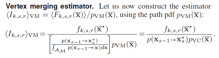
Path pdf
- 由 VM 产生的路径 \(p_{VM}(\bar{\mathrm{x}})\) 的 pdf 如下
\[ p_{VM}(\bar{\mathrm{x}})=P_{acc}(\bar{\mathrm{x}})p_{VC}(\bar{\mathrm{x}}) \]
- \(p_{VC}(\bar{\mathrm{x}})\)
表示直接将两条 subpath 连接在一起的 pdf,连接端点 \({\mathrm{x}}_{s-1},{\mathrm{x}}_{s}\)
- 表达形式见第 3 部分
- \(P_{acc}(\bar{\mathrm{x}})\)
表示这样一条路径可接受的概率
- \(P_{acc}(\bar{\mathrm{x}})\le1\)
\[ \begin{aligned} P_{acc}(\bar{\mathrm{x}})\ &=\ \mathrm{Pr}(\Vert\mathrm{x}_s-\mathrm{x}^\ast_{s}\Vert^2<r)\\ &=\ \int_{\mathcal{A}_\mathcal{M}}p(\mathrm{x}_{s-1}\to\mathrm{x})d\mathrm{x}\\ &\approx|{\mathcal{A}}_{\mathcal{M}}|p(\mathrm{x}_{s-1}\to\mathrm{x}^\ast_s)\\ \end{aligned} \]
- \({\mathcal{A}}_{\mathcal{M}}=\left\{\mathrm{x}\in \mathcal{M}|\Vert\mathrm{x}_s-\mathrm{x}\Vert^2<r\right\}\):核半径之内
- 我们假设 \({\mathcal{A}}_{\mathcal{M}}\) 内部的 pdf
是一个常数
- PPM 也是这么假设的
- [Hachisuka et al. 2008]
- 渐进分析
- [Knaus and Zwicker 2011].
- PPM 也是这么假设的
- 我们假设 \({\mathcal{A}}_{\mathcal{M}}\) 是一个半径为 \(r\) 的圆
- 如果现实和我们假设不符,这样可能会导致估计不准确
- areas of geometric variation and when p is far from constant
- \({\mathcal{A}}_{\mathcal{M}}\)
内部的 pdf 不是常数,
- \(\mathrm{x}_{s-1}\) 的 BSDF 是 glossy 的
- 几何变异大
- \(r\) 趋向于 0 的时候就是准确的
- \(\mathrm{x}_{s-1}\) 如果是镜面,而且恰好 \(\mathrm{x}_s^{\ast}\) 落在区域内部,则 \(P_{acc}=1\)
- 最终估计如下
\[ p_{VM}(\bar{\mathrm{x}})=\left[\pi r^2\ p(\mathrm{x}_{s-1}\to\mathrm{x}^\ast_s)\right](\bar{\mathrm{x}})p_{VC}(\bar{\mathrm{x}}) \]
4.1 Efficiency of Different Path Sampling Techniques
- 启发式的指数因子的加入源于这样的一种观察,pdf
较大的区域,方差估计较小
- a higher pdf most often results in a lower variance estimate
Sampling densities
- \(P_{acc}(\bar{\mathrm{x}})\le1\),说明 VM 的路径 pdf 最大不会超过 VC 的的 pdf
- VM 的操作相当于在 \(\mathrm{x}_{s-1}\) 的一个立体角中采样
- 如果 \(\mathrm{x}_{s-1}\) 是 diffuse 材质的,那么结果应该和立体角中采样是一样的
- The resulting VM path pdf \(p_{VM}\) can then be six or more orders of magnitude lower than the corresponding VC pdf
- 当 \({\mathcal{A}}_{\mathcal{M}}\)
区域和光源相近时,VM 的 pdf 和单项采样的 pdf 几乎相等
- unidirectional sampling (US) and VM can have almost equal pdfs.
- 直观上的理解,击中光源的概率和击中 \({\mathcal{A}}_{\mathcal{M}}\) 的概率一致
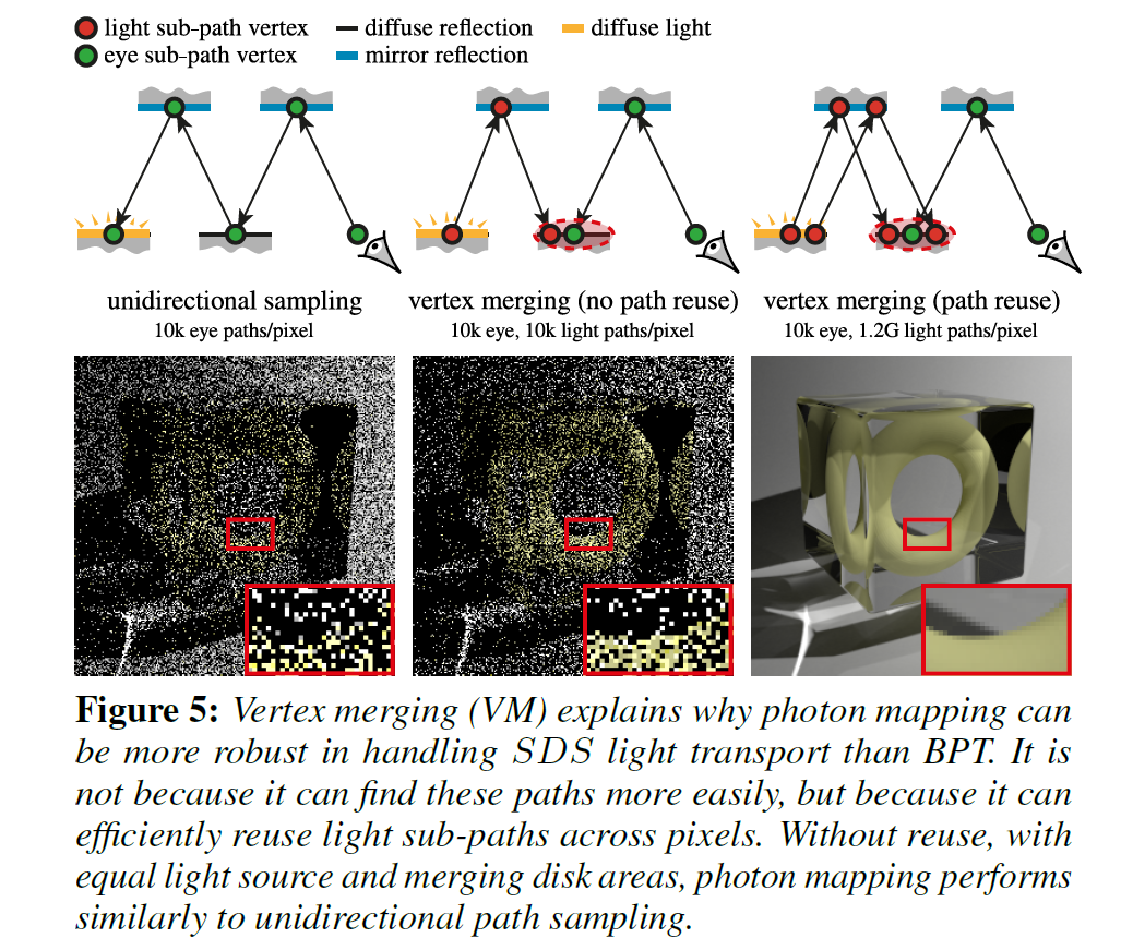
Path reuse efficiency
- PM 在采样上效率可能并不是比 BPT 更高,但是计算上效率更高
- the power of VM is its
computational efficiency
- the power of VM is its
- PM 效率高的原因在于它能够用上很多之前不能使用的 light subpath
- It performs conditional path concatenation, which is as cheap as neighborhood checking. This enables the reuse of a large number of light sub-paths at the cost of a single range search.
- 不搜索的话(只用一条路径),就找不到更多的路径
- 没有 reuse 的话,PM 效果并不好
5. A Combined Light Transport Algorithm
- 算法
- 我们已经将 PM 描述成一个一个采样过程,可以直接利用 MIS 将 PM 和 BPT 结合在一起
- 长度为 k 的路径,BPT 提供了 k+1 种采样途径,PM
额外提供了 k-1 种采样途径
- 实际操作中我们对端点不做连接处理
- 所以只会在中间的 k-1 个顶点处进行 PM
- 这一部分我们使用一个固定大小的 \(r\),这样子的结果是有偏的
5.1 Mathematical Formulation
\[ I=\int_{\Omega}f(x)d\mu(x) \]
- 使用 MIS 结合 BPT(VC) 和 PM(VM)估计上述值
\[ \begin{aligned} \langle I\rangle_{MIS}&=C_{VC}+C_{VM}\\ &=\dfrac{1}{n_{VC}}\sum_{l=1}^{n_{VC}}\sum_{s\ge0,t\ge0}w_{VC,s,t}(\bar{\mathrm{x}}_l)\langle I\rangle_{VC}(\bar{\mathrm{x}}_l)\\ &+\dfrac{1}{n_{VM}}\sum_{l=1}^{n_{VC}}\sum_{s\ge2,t\ge2}w_{VM,s,t}(\bar{\mathrm{x}}_l)\langle I\rangle_{VM}(\bar{\mathrm{x}}_l) \end{aligned} \]
- s:light subpath 的结点数
- t:eye subpath 的结点数
- 权重设置如下(v can be VC or VM)
\[ w_{v,s,t}(\bar{\mathrm{x}})=\dfrac{n_v^\beta p_{v,s,t}^\beta(\bar{\mathrm{x}})}{n_{VC}^\beta\sum_{s'\ge0,t'\ge0} p_{VC,s',t'}^\beta(\bar{\mathrm{x}})+n_{VM}^\beta\sum_{s'\ge2,t'\ge2} p_{VM,s',t'}^\beta(\bar{\mathrm{x}})} \]
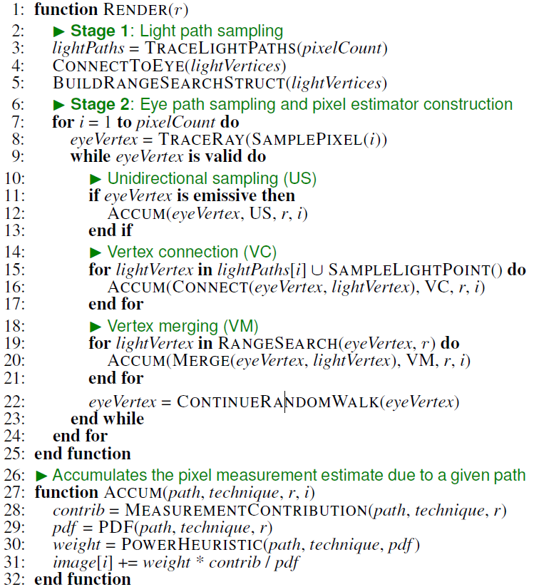
5.2 Implementation
- 采样的代价很大
- The BPT implementation according to Veach [1997] reuses sub-paths by connecting every eye sub-path vertex to every vertex on one light sub-path.
- thanks to the low cost of range query, an eye sub-path vertex can be potentially merged with vertices of a large number of pre-generated light sub-paths.
- 为了提高复用率,我们把算法分为两个阶段
- sampling of the light and eye sub-paths
- L:11-13
- 看当前结点是否自发光,如果自发光,则收集 radiance
- 为了减少相关性,我们不保存 light subpath
的第一个顶点位置,修改为重新对它随机采样
- To reduce correlation, we follow Veach [1997] and do not store the first vertex of a light sub-path, instead connecting every eye vertex to a new, randomly sampled point on a light source.
- 评估权重的时候,把信息存储在节点上以提高效率
- Most of the terms required to evaluate path contributions and pdfs are stored with the sub-path vertices for improved efficiency.
- 伪代码如下
6. Achieving Consistency
- 我们的方法是有偏的(blur),但是是一致的
- 通过渐进的减小半径 r 、累计所有的结果实现
- 最终的结果通过前 N 次独立的采样渲染结果平均得到
- 每一轮的计算和上面提到的单次估计相同(5.1)
\[ \langle I\rangle_{VCM}=\dfrac{1}{N}\sum_{i=1}^N(C_{VC,i}+C_{VM,i}) \]
- 每一轮新的迭代使用新的 eye subpath 以及 light subpath,减小半径
- \(r_i=r_1\sqrt{i^{\alpha-1}}\), where \(\alpha\in(0,1)\)
6.1 Asymptotic Error Analysis
- 方差渐进分析
- MSE
- BPT:\(O(\dfrac{1}{N})\)
- PPM:\(O(\dfrac{1}{N^\frac{2}{3}}),\alpha=\dfrac23\)
- 理论上我们的 MSE 应该介于上面两者之间
- VC:无偏的
\[ \mathrm{Var}[\langle I\rangle_{VC}]=O(1),\ \mathrm{Bias}[\langle I\rangle_{VC}]=0 \]
- VM:借用 Knaus and Zwicker [2011] 的结论
- 半径缩减采用上面的方案
\[ \mathrm{Var}[\langle I\rangle_{VM}]=O(\dfrac{1}{r^2_i}),\ \mathrm{Bias}[\langle I\rangle_{VM}]=O(r_i^2) \]
\[ \mathrm{Var}[\langle I\rangle_{VM}]=O(i^{1-\alpha}),\ \mathrm{Bias}[\langle I\rangle_{VM}]=O(i^{\alpha-1}) \]
- 计算各种参数的量级
- \(p_{VC,s,t}(\mathrm{x})=O(1)\)
- \(p_{VM,s,t}(\mathrm{x})=O(r_i^2)=O(i^{\alpha-1})\)
- \(w_{VC,s,t}(\bar{\mathrm{x}})=\dfrac{O(1)}{O(1)+O(i^{\beta(\alpha-1)})}=O(1)\)
- \(\alpha\in(0,1)\)
- \(w_{VM,s,t}(\bar{\mathrm{x}})=\dfrac{O(i^{\beta(\alpha-1)})}{O(i^{\beta(\alpha-1)})+O(1)}=O(i^{\beta(\alpha-1)})\)
- \(\alpha\in(0,1)\)
Variance
- 方差估计,由于每一步的采样都是独立的
\[ \mathrm{Var}[\langle I\rangle_{VCM}]=\dfrac{1}{N^2}\sum_{i=1}^N(\mathrm{Var}[C_{VC,i}]+\mathrm{Var}[C_{VM,i}]) \]
- VC,VM 认为是独立采样,所以能拆开
- 我们假定 \(2\beta(\alpha-1)-\alpha<-1\)
- 实际操作我们会让 \(\beta\ge1\),所以能保证
\[ \begin{aligned} &\mathrm{Var}[\langle I\rangle_{VCM}]\\ =&\dfrac{1}{N^2}\sum_{i=1}^N\left(O(1)O(1)+O(i^{2\beta(\alpha-1)})O(i^{1-\alpha})\right)\\ =&O(N^{-1})+O(i^{2\beta(\alpha-1)-\alpha})\\ =&O(N^{-1})\\ \end{aligned} \]
Bias
- 类似的估计
\[ \begin{aligned} &\mathrm{Bias}[\langle I\rangle_{VCM}]\\ =&\dfrac{1}{N}\sum_{i=1}^N(\mathrm{Bias}[C_{VC,i}]+\mathrm{Bias}[C_{VC,i}])\\ =&O(i^{(\beta+1)(\alpha-1)})\\ \end{aligned} \]
MSE
- 假定 \(\alpha\le\dfrac{2\beta+1}{2\beta+2}\)
\[ \begin{aligned} &\mathrm{MSE}[\langle I\rangle_{VCM}]\\ =&\mathrm{Var}[\langle I\rangle_{VCM}]+\mathrm{Bias}^2[\langle I\rangle_{VCM}]\\ =&O(N^{-1})+O(N^{2(\beta+1)(\alpha-1)})\\ =&O(N^{-1})\\ \end{aligned} \]
- 令 \(\beta=1\),此时对于任意的 \(\alpha\in(0,0.75)\) 都满足上面的条件
- 比 PPM 更快
- PPM 的估计如下
\[ \begin{aligned} &\mathrm{MSE}[\langle I\rangle_{VCM}]\\ =&\mathrm{Var}[\langle I\rangle_{VCM}]+\mathrm{Bias}^2[\langle I\rangle_{VCM}]\\ =&O(N^{-\alpha})+O(N^{2(\alpha-1)})\\ \le&O(N^{-\frac{2}{3}})\\ \end{aligned} \]
Discussion
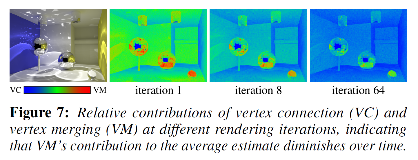
- 收敛更快,直观上我们可以理解为 VM 随着跌打的增加贡献逐渐减小,几乎等同于 BPT
- VM 初始方差更小,于是能够在有限的样本内很快得到一张可以接受的图片
7.Result
- 很多效果图
8.DIscussion
- 参数选择:\(r1\):0:01%-0:07% of
the scene’s bounding box,\(\alpha=\dfrac{2}{3}\)
- 为了做对比实验
- 实际使用的时候,建议参数
- VCM we recommend setting \(r1\) smaller than for PPM and \(\alpha=0.75\)
- 限制
- 不好处理点光源,不能采样
- 对于 PM 和 BPT 都不能很好处理的场景,VCM 也不能很好的处理
- caustics falling on a highly glossy surface
A Additional Vertex Merging Derivations
A.1 Contribution Function for Extended Paths
PM pixel measurement estimator.
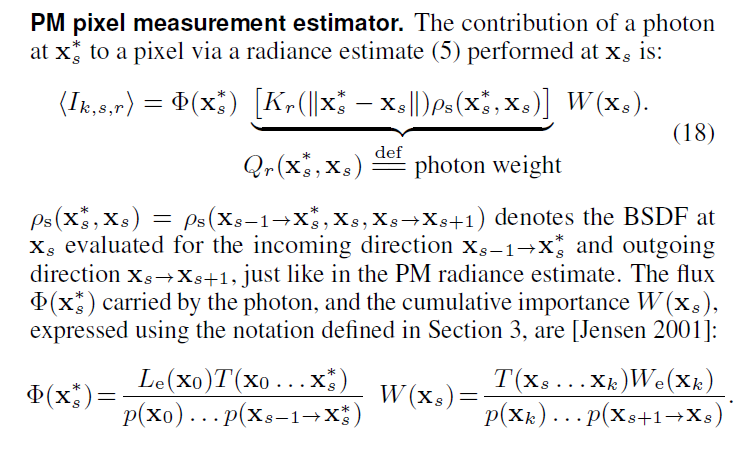
Path integral and contribution function
- \(Q\) 项中的 \(K\) (kernel)会引发模糊现象
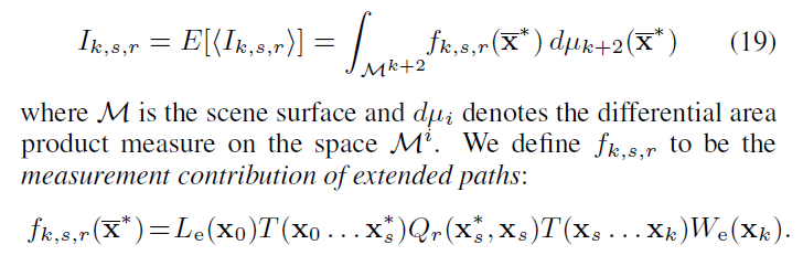
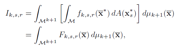
A.2 Reducing the Path Integral Dimension
- 拆解为两部分,正常采样 + 贡献项
- equation (20)
- 贡献项的计算
- MC 估计即可
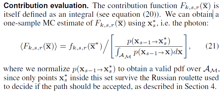
- VM 的估计