(论文)[2020-SIG] Path Cuts, Efficient Rendering of Pure Specular Light Transport
Path Cuts: Efficient Rendering of Pure Specular Light Transport
Key Words
- 点光源,针孔摄像机,pure specular,multi-bounce,path-space
- reflections and refractions
- 反射和折射
1. Introduction
- 传统的渲染方法,蒙特卡洛方法找到一条从光源到相机的路径
- none of them are able to find multi-bounce pure specular light paths from a point light to a pinhole camera
- 之前的方法
- 初始化为一条不可接受的的路径(可能是不太正确的路径,但是很接近最终解)
- 根据求解器求解出一条正确的路径(牛顿法)
- 可以解决,但是有局部性问题
- Walter’s method:全局的方法
- using a hierarchical data structure on top of meshes with interpolated normals, but only works for a single refraction.
- 论文的方法
- we enumerate the discrete set of admissible pure specular paths of a given length and type connecting the light and the camera. We globally slice the path space into small regions
- within a region we solve the local problem of refining the path to become admissible
- 解决的问题
- We use a path space hierarchy combined with interval arithmetic
bounds to efficiently prune non-contributing regions of path space, and
to slice the path space into regions small enough that local refinement
becomes feasible.
- 路径空间划分,剪枝,每个小区域求局部解
- We use an automatic differentiation tool and a Newton-based solver
to find an admissible specular path within a given path space region,
and splat its contribution onto the image plane.
- 自动微分工具,基于牛顿法的求解器
- 给定一个区域内的求解,然后在全局上加入它的贡献
- We show that our purely specular solution can be used to initialize
paths for other algorithms, such as an MCMC-based approach to render
with small but non-zero roughness.
- 论文算法的到的路径可以用于其他算法初始值的设定
- We use a path space hierarchy combined with interval arithmetic
bounds to efficiently prune non-contributing regions of path space, and
to slice the path space into regions small enough that local refinement
becomes feasible.
- 评价
- ours is the first approach to directly focus on multi-bounce purely specular paths on complex geometric surfaces given by triangle meshes with interpolated normals.
2. 相关工作
- 费马原理,牛顿法求解中间结点
- 优化问题,最大化/最小化长度
- Walter
- 费马定理在现实场景中不太使用(图元的不同法线、几何)
- the admissible paths are simply the ones whose vertices align the normal vector with the (refractive) half vector.
- limited to a single refractive surface event
- 不容易扩展到 k-bounce
- Markov chain Monte Carlo
- this method does not work for pure specular paths
- and requires the Markov chain light transport setting to be applicable.
- Manifold next event estimation (MNEE)
- the method can connect any shading point on a non-specular surface, through one or more refractions, to a light source sample.
- 没有全局搜索
- 存在局部性问题,多解则不能很好工作
- half vector space light transport (HSLT)
- a path is represented by its start and end point constraints and a sequence of generalized half vectors
- HSLT does not require a specular/non-specular classification of the path vertices
- 最近的工作
- Recently, concurrent work by Zeltner et al. [2020] presented a specular manifold sampling technique, which is able to handle glints, reflective/refractive caustics, and specular-diffuse-specular light transport
- 解决闪烁,焦散问题
- Interval arithmetic
- Glint rendering methods
- Lightcuts
- 虚拟光源
- 层次结构
- Inspired by the idea of lightcuts, we propose path cuts to organize all the triangles, whether geometric or tessellated from bump/normal maps, into a hierarchy.
- We use the path cuts to efficiently prune non-contributing areas of the path space; i.e. regions where the alignment of the normal and half vectors is guaranteed to be impossible.
3. PATH SPACE TRAVERSAL USING PATH CUTS
- For each number of bounces k the problem needs to be solved independently
- different path types of a given length are themselves independent.
基本量
- k-bounces
- path vertices:k+2
- light(L),k-bounces,pinhole camera(E)
- k+1 segments
- path vertices:k+2
- bounce point:\(x_i\)
- 场景由 n 个带有插值法线的三角形组成 \(T_i\)
- scene surface:\(\mathcal{M}\)
思路
- Our idea is to first isolate all k-tuples of triangles that could give rise to an admissible path, then find those paths within the k-tuple using a root solver. In this section, we focus on the first part, finding potentially contributing k-tuples of triangles.
- then find those paths within the k-tuple using a root solver.
- In this section, we focus on the first part, finding potentially contributing k-tuples of triangles.
3.1 Path cuts for hierarchical pruning
- brute-force:暴搜
- \(O(n^k)\)
- 树层次结构 tree hierarchy \(\mathcal{H}\)
- Each node \(S_i\in\mathcal{H}\) represents a surface patch on \(\mathcal{M}\), and records the 3D interval (bounding box) \(N_i\) of all surface normals and the 3D interval (bounding box) \(P_i\) of all surface positions in this patch.
- Note that this "root" path cut is for the entire image, as our method is independent of pixels.
- 找路径时考虑 \(\mathcal{H^k}=\mathcal{H}\times\mathcal{H}\times\cdots\times\mathcal{H}\)
- 假使我们选中了 \((S_{j_1},\cdots,S_{j_K})\in\mathcal{H^k}\)
- “thick path”
- the set of all paths from the light to the camera whose vertices are within the corresponding nodes
- 恰好在上面的结点中
\[ L\to(x_1\in S_{j_1})\to(x_2\in S_{j_2})\to\cdots\to(x_k\in S_{j_k})\to E \]
- We denote such a “thick path” as a path cut, in analogy to multidimensional lightcuts.
Insight
- if we can quickly determine whether a path cut potentially contains an admissible specular path, we can use this information to prune the path space to quickly converge to contributing paths.
- 怎么判断 path cut 是否含有一个可接受的结果(specular path)?
- conservative(保守)
- existence of one or more admissible paths has to be always correctly detected.
- The reverse need not be true: if we cannot prove non-existence, we can always subdivide the path cut.
3.2 Validating a path cut
- a pure specular path is admissible
- at each surface bounce, the normal vector is aligned with the (reflective or refractive) half vector.
- test locally
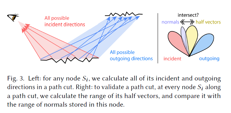
- interval arithmetic:区间算术
- 对于层次结构中的结点 \(S_i\)
做包围盒(AABB)
- \(P_i\) :\(S_i\) 中点的位置
- \(N_i\):\(S_i\) 中法线的位置
- 所有可能的从 \(S_{i-1}\) 到 \(S_i\) 的入射方向、出射方向
- \(D_{in}^i=normalize(P_{i-1} −P_i)\)
- \(D_{out}^i=-D_{in}^{i+1}=normalize(P_{i+1}−P_i)\)
- half vector
- \(H_i=normalize(D_{out}^i+D_{in}^i)\)
- 判断 \(H_i\bigcap N_i\) 是否为空,即可判断是否存在法线和半角矢量对齐(相等)
- 对每一次 bounce 做上面的判断,如果存在一个 \(i\) 使得 \(H_i\bigcap N_i\)
为空,那么不可能产生一条可行的光路
- 剪枝 prun
3.3 Subdividing a path cut
- Once we know that a path cut has potential to contribute a pure
specular path, we subdivide this path cut.
- 如果一条 path cut 有可能产生纯反射光路,则对其进行细分
细分方式
(1)简单的细分
- 把所有的非叶子结点都展开
- 复杂度变回去了,很高
(2)随机选择一个非叶子结点进行展开
(3)展开最大的结点
- largest bounding box
- 确实很直观
(4)展开 \(H_i\bigcap N_i\) 区间最大的结点
- 实验验证效果不好,能够看见比方法(3)更多的结点
细分结束
- As we repeat the subdivision process, finally we will end up with path cuts that consist of only leaf nodes, i.e. one triangle per bounce.
一个细分的问题
- 怎么处理细分,结点数变化怎么处理,分成两条
path cut 吗?
- 感觉确实没问题,复杂度也不高,只需要检查当前展开的结点和两边结点的连接关系即可
4. SOLVING FOR A SPECULAR LIGHT PATH
- 现在的结果是找到了一条 path cut,每个结点都是三角形
\[ L\to(x_1\in T_1)\to(x_2\in T_2)\to\cdots\to(x_k\in T_k)\to E \]
- 现在的问题
- find its contribution to the image plane
- 也就是说找到光路
4.1 Finding an admissible path
- Finding such a light path is trivial if the triangles are
flat mirrors (i.e. they do not have interpolated
shading normals distinct from the geometric normal).
- We just need to repeatedly take the virtual image of the point light across the plane containing \(T_i\) and finally connect it to the camera.
- 把光源 \(L\) 做 \(T_1\) 的虚像得到 \(I_1\),然后把 \(I_1\) 做 \(T_2\) 的虚像得到 \(I_2\),重复这个过程得到 \(I_K\),连接 \(I_K\) 和 \(E\) 即可得到光路
- 平面镜成像原理
- However, this does not cover common situations with
refractions and normal interpolation
(curvature).
- curvature:曲率
- In the general case, we need to find the vertex locations using a root solver.
- 使用重心坐标系 \(\alpha_i,\beta_i,\gamma_i\)
- \(\alpha_i+\beta_i+\gamma_i=1\)
- 知道了 \(\alpha_i,\beta_i\) 可以通过三个顶点插值出法线 \(n_i(\alpha_i,\beta_i)\) 和顶点的位置 \(x_i(\alpha_i,\beta_i)\)
- 继而可以求出入射光线的方向 \(normalize(x_{i-1}-x_i)\),入射光线的方向 \(normalize(x_{i+1}-x_i)\)
- 接着求出半角矢量 \(h_i(\alpha_i,\beta_i)\)
- 感觉不太对,应该是下面这个,但是不影响
- \({\color{red}h_i(\alpha_i,\beta_i,\alpha_{i-1},\beta_{i-1},\alpha_{i+1},\beta_{i+1})}\)
- 半角矢量可以应用在反射和折射上面
- 感觉不太对,应该是下面这个,但是不影响
- 按照惯例,我们假设法线和半角矢量指向折射率较低的介质(一般但不一定是空气)
- 约束条件:逐渐缩小如下值(希望相等)
- \(C_i(\alpha_i,\beta_i)=\mathrm{n}_i(\alpha_i,\beta_i)-\mathrm{h}_i(\alpha_i,\beta_i)\)
- 在三角形内部
- \(\alpha_i\ge0,\beta_i\ge0,\alpha_i+\beta_i\le1\)
- 整条路径的限制条件
\[ C(\alpha_1,\beta_1,\cdots,\alpha_k,\beta_k)=(C_1,C_2,\cdots,C_k) \]
- the constraint function has 2k variables and 3k output values.
- An alternative with 2k output values can be defined by projecting the normals and half vectors into the local geometric space, and dropping their 𝑧 coordinates. We found this alternative formulation gives equivalent results and is slightly slower due to the extra vector transformations.
- Newton iteration
- This requires solving a 3k × 2k linear system, in the least-squares sense, at each iteration.
- 限制迭代次数
- We bound the maximum number of iterations to 5.
- If after reaching the maximum terations, the resulting vertices are not all within their respective triangles, we assume there is no solution.
- 求解出来之后,我们对相邻的两个三角形做可见性测试
- The visibility test can be skipped for objects known to be convex.
- 为什么不需要
4.2 The contribution of an admissible path
- 影响强度的因素
- The contribution of the path to the image consists of the product of
several terms:
- visibility (already handled above)
- light intensity
- the product of Fresnel terms along the path
- volumetric absorption
- the generalized geometry term
- and the pixel importance function value
- The contribution of the path to the image consists of the product of
several terms:
- 这里只考虑最后两个因素(其他不需要在这里讨论)
- precisely define our camera model as a pinhole camera, with a sensor plane at a distance of 1 world unit from the camera position (pinhole)
- For the purposes of the explanation below, the camera endpoint P of the path is thus on the sensor, not on the pinhole C itself.
Pixel importance function value
- Consider a ray \((P,\omega)\) leaving the sensor point \(P\) in direction \(\omega = normalize(C-P)\)
- \(W_{ij}(P,\omega)\)
- We will need to include the corresponding \(W_{ij}\) in the path contribution
- \(W_{ij}\) 对谁归一化(和为1)
- These units cannot be pixels, otherwise the brightness of specular contributions would change with image resolution.
- Instead, we find that the normalization has to be with respect to real world units, on the image sensor at a distance of 1 unit from C.
- if the horizontal field-of- view is \(\theta\) and the aspect ratio
(height/width) is \(r\) , the area of
the image plane in world units is \(A\)
- \(A=4r\tan^2(\dfrac{\theta}{2})\)
- 归一化
- \(W_{ij}(P,\omega)=\dfrac{K_{ij}mn}{A}\)
- 像素分辨率 \(m\times n\)
- Here we first define \(K_{ij}\) to be the pixel reconstruction filter normalized in pixel units,
- and then include the additional factor of \(\dfrac{mn}{A}\) to make \(W_{ij}\) normalized in world units.
- \(W_{ij}(P,\omega)=\dfrac{K_{ij}mn}{A}\)
- 图形学渲染:radiance meter
- brightness to change with image resolution
- 实际的摄像机:photon counter
- brightness to change with image resolution
Generalized geometry term(GGT)
- 这部分暂时没啥看懂
- "intensity" or "distance correction factor"
- Consider the ray propagation function \(F:\mathbb{R^2}\to\mathbb{R^2}\) that maps a neighborhood of the camera sensor point \(P\) through the admissible specular path \(\bar{x}\) to the imaginary plane crossing the point light position, orthogonal to the last path segment. The GGT is the value
\[ G(\bar{x})=\dfrac{1}{|\det J_F(P)|} \]
- We initialize position differentials \(P_x\) and \(P_y\) of unit length on the camera sensor plane, and trace them along the specular path to the imaginary plane crossing the point light position, orthogonal to the last path segment, finding the final position differentials \(L_x\) and \(L_y\). Finally, we can compute the GGT as
\[ G(\bar{x})=\dfrac{1}{|L_x\times L_y|} \]
- \(|L_x\times L_y|\)
很小,结果不真实
- \(|L_x\times L_y|\approx||L_x||\cdot||L_y||\cdot\max\{\epsilon,|normalize(L_y)\times normalize(L_y)|),\}\)
- A value of \(\epsilon = 0.01\) works well in general.
- We observe that this regularization solves the issue of occasional very bright glints, while not affecting the remaining glints.
4.3 Multiple solutions
- 解可能不止一个
- 虽然我们实验上都是得到一个解,但是这不一定理论正确
Finding all discrete solutions
- 问题
- Even if a single solution exists, standard Newton’s method still
does not theoretically guarantee that the solution will be found.
- 一个解但是没找到
- Furthermore, there is a possibility of multiple discrete solutions
- 多个解
- Even if a single solution exists, standard Newton’s method still
does not theoretically guarantee that the solution will be found.
- Both of these issues can be theoretically handled with the interval version of Newton’s method, as suggested by Mitchell and Hanrahan [1992] and Walter [2009].
- 我们实验发现差不多
- 可能的解释
- our meshes already subdivided to small enough triangles, so multiple solutions within a single triangle do not frequently occur in practice
Infinite solution regions
- 圆柱体,内部纯反射,光源和针孔摄像机放置在两头,中间的圆给出无穷多个解
- 无法求解
- 法线并非插值得到
- 只能求解三角形,而且内部的法线是由插值得到的图形
7. CONCLUSION AND FUTURE WORK
- We use a path space hierarchy combined with interval arithmetic bounds to efficiently prune non-contributing regions of path space, and to slice the path space into small region where the search problem becomes local. Finally, we isolate admissible specular paths by a Newton solver applied to a constraint function, whose gradients are computed by automatic differentiation.We discuss in detail how such discovered paths should contribute to the image plane.
作者报告
- 视频:https://www.bilibili.com/video/BV1Mi4y1N7Np
- 南京理工大学 王贝贝
- GAMES 链接:http://games-cn.org/games-webinar-20210401-177/
- 代码:https://github.com/wangningbei/mbglints
notes
现有的方法解决不能解决问题
- BDPT:很难在交汇处实现完美的镜面反射。折射
- MLT:思路是在一开始的种子路径上,使用小的偏移找到新的路径
- 一开始的种子路径很难找到
论文的方法是确定性的结果,是没有噪声的
我们的方法可以作为 MLT 的种子路径
只能支持点光源
展示是基于 CPU
问题
- bounce 比较多的时候,搜索代价变大
- 论文最多 4-bounces
- 牛顿法不能求出所有解
- 区间牛顿法可以,但是代价大
- 划分区间,用一个条件判断使得否只有唯一解,如果只有唯一解,利用牛顿法求解,否则继续细分
- AABB 包围盒比较松,在做法线和半角矢量是否有交判断中比较松(不能提前排除无解可能性)