(论文)[2023] 基于子空间的双向路径连接渲染技术(4)
基于子空间的双向路径连接渲染技术(4)
代理追踪技术
倒数的无偏估计方法
参数推荐配置
\[ r(\bar{x})=\left\vert{1-\dfrac{f(x_{k-1})}{Bq(x_{k-1})}}\right\vert \]
\[ B=\max\left(\dfrac{f(x)}{q(x)}\right) \]
- 此时只有 RR,没有 Splitting
RRS 参数
- 构造随机变量
\[ \tilde{Y}'=\dfrac{g(X)}{B}+\dfrac{g(X)}{r(X)}\sum_{i=1}^{r(X)}\tilde{Y}_i' \quad\quad(4.9) \]
\[ g(X) = 1 - \dfrac{f(X)}{Bp(X)} \]
- \(\{\tilde{Y}_i'\}\):独立同分布的多个随机变量 \(\tilde{Y}'\) 的集合
- \(r(X)\) 可能为小数,此时
- 整数时则不需要展开
- 样本数:\((0,1]\to1,(1,2]\to2,\cdots\)
\[ \sum_{i=1}^{r(X)}\tilde{Y}_i' =\sum_{i=1}^{\lfloor{r(X)}\rfloor}\tilde{Y}_i'+\tilde{Y}_i'^{\ast} \]
\[ \tilde{Y}_i'^{\ast}= \left\{ \begin{array}{rrl} \tilde{Y}_{\lceil{r}\rceil}',&\text{probability}&r-\lfloor{r}\rfloor\\ 0,&\text{probability}&\lceil{r}\rceil-r\\ \end{array} \right. \]
- 求和符号 \(\sum_{i=0}^{\lfloor{r(X)}\rfloor}\) 和 \(r(X)\) 都是为了描述 RRS 的
- \(E\left[\tilde{Y}\right]\) 就是 \(\alpha\) 的无偏估计
\[ \tilde{Y}=\tilde{Y}'+\dfrac{1}{B} \]
- 可以发现与前缀路径 \(\bar{Z}\) 无关
\[ r(X\vert \bar{Z})=r(X) \]
RR 简单分析
- 如果只看 RR
\[ \begin{aligned} \tilde{Y}' &=\dfrac{g(X)}{B}+\dfrac{g(X)}{r(X)}\tilde{Y}_i'^{\ast}\\ &=\dfrac{g(X)}{B}+\dfrac{g(X)}{r(X)}\cdot r(X)\cdot\tilde{Y}_i'\\ &=\dfrac{g(X)}{B}+g(X)\tilde{Y}_i'\\ \end{aligned} \]
- 此时
\[ E\left[\tilde{Y}\right]=\int\left(\dfrac{g(x)}{B}+g(x)\cdot E\left[\tilde{Y}\right]\right)p(x)\;\mathrm{d}x \]
\[ E\left[\tilde{Y}'\right]=\alpha-\dfrac{1}{B} \]
- RRS 是每次多得了好几个样本,总体需要再除以得到的样本数
- 即除以 \(r(X)\)
改造
- 方便估计
- 构造 \(Y\) 如下
\[ Y=\dfrac{1}{B}+\dfrac{g(X)}{r(X)}\sum_{i=1}^{r(X)}Y_i \]
- 类似的我们能够得到期望为 \(\alpha\)
- 可得:\(Y\) 的方差比 \(\tilde{Y}'\) 大
- 辅助随机变量 \(Y'\),\(\dfrac{1}{B}\) 是常数,于是 \(Y'\) 和 \(Y\) 方差相同
\[ Y'=Y-\dfrac{1}{B} \]
- 带入,于是有
\[ Y'+\dfrac{1}{B}=\dfrac{1}{B}+\dfrac{g(X)}{r(X)}\sum_{i=1}^{r(X)}\left(Y_i'+\dfrac{1}{B}\right) \]
\[ Y'=\dfrac{g(X)}{r(X)}\sum_{i=1}^{r(X)}\left(Y_i'+\dfrac{1}{B}\right) \quad\quad(4.11) \]
- 公式 \(4.9\) 和 \(4.11\) 的区别在于 \(\dfrac{g(X)}{B}\) 的处理不同
- \(\tilde{Y}'\) 直接加到结果
- \(Y'\) 放到了 RRS 的多次求和中
- 因此
\[ Var\left(Y\right) =Var\left(Y'\right) \ge Var\left(\tilde{Y}'\right) =Var\left(\tilde{Y}\right) \]
- 通过最小化 \(Y\) 的方差上界去优化
\(\tilde{Y}\) 的方差上界
- \(Y\) 更容易处理
上界
- 当 \(r\) 为整数的时候,\(Y_i\) 独立
\[ E\left[\left(\sum_{i=1}^{r}Y_i\right)^2\right]=rE[Y^2]+(r^2-r)E^2[Y] \]
- 我们认为 \(r\)
为正实数的时候,\(E\left[\left(\sum_{i=1}^{r}Y_i\right)^2\right]\)
也保持着上面的变化规律
- EARS(SIG22) 论文中也是这么用的
- 根据这一个近似,可以得到
- \(X,Y\) 独立
- 记号:\(V[Y]:Var[Y]\)
\[ \begin{aligned} V[Y] &=V\left[Y-\dfrac{1}{B}\right]\\ &=E\left[\left(Y-\dfrac{1}{B}\right)^2\right]-E^2\left[Y-\dfrac{1}{B}\right]\\ &=E\left[\dfrac{g^2(X)}{r^2(X)}\left(\sum_{i=1}^{r(X)}Y_i\right)^2\right]-\left(E\left[Y\right]-\dfrac{1}{B}\right)^2\\ &=E\left[\dfrac{g^2(X)}{r^2(X)}\left(\sum_{i=1}^{r(X)}Y_i\right)^2\right]-\left(E\left[Y\right]-\dfrac{1}{B}\right)^2\\ &\approx E\left[\dfrac{g^2(X)}{r^2(X)}\left(r(X)E[Y^2]+(r^2(X)-r(X))E^2[Y]\right)\right]-\left(E\left[Y\right]-\dfrac{1}{B}\right)^2\\ &=E\left[\dfrac{g^2(X)}{r(X)}\left(V[Y]+r(X)E^2[Y]\right)\right]-\left(E\left[Y\right]-\dfrac{1}{B}\right)^2\\\ &=E\left[\dfrac{g^2(X)}{r(X)}\right]V[Y]+E\left[g^2(X)\right]E^2[Y]-\left(E\left[Y\right]-\dfrac{1}{B}\right)^2\\\ \end{aligned} \]
- 将与 \(r(x)\) 无关的常数定义为 \(c_0\)
\[ c_0=E\left[g^2(X)\right]E^2[Y]-\left(E\left[Y\right]-\dfrac{1}{B}\right)^2 \]
\[ V[Y]=E\left[\dfrac{g^2(X)}{r(X)}\right]V[Y]+c_0 \]
\[ V[Y]=\dfrac{c_0}{1-E\left[\dfrac{g^2(X)}{r(X)}\right]} \]
- 定义效率 \(\text{Eff}\),我们试图最大化 \(\text{Eff}\)
- 因为方差 \(\propto\dfrac{1}{N}\),\(N\) 为样本数
\[ \text{Eff}=\dfrac{1}{C\times V[Y]} \]
- 我们认为开销正比于从 \(p(\cdot)\)
中采样的次数,于是得到
- 每次 \(Y\) 的采样,带来期望 \(E[r(x)]\) 次分裂
\[ C=\dfrac{1}{1-E[r(x)]} \]
- 第 \(i\) 层的采样次数个数:\(E^{i-1}[r(x)]\)
\[ 1+E[r(x)]+E^2[r(x)]+\cdots=\dfrac{1}{1-E[r(x)]} \]
- 于是
\[ \begin{aligned} \text{Eff} &=\left(1-E[r(x)]\right)\cdot\dfrac{1}{c_0}\cdot\left({1-E\left[\dfrac{g^2(X)}{r(X)}\right]}\right)\\ &=\dfrac{1}{c_0}\left(1-\int r(x)p(x)\;\mathrm{d}x\right)\cdot\left({1-\int \dfrac{g^2(x)}{r(x)}p(x)\;\mathrm{d}x}\right)\\ &\le\dfrac{1}{c_0}\left(1-\int \vert{g(x)}\vert p(x)\;\mathrm{d}x\right)^2 \end{aligned} \]
- 取等条件
\[ r(x)p(x)\equiv\dfrac{g^2(x)}{r(x)}p(x)\Rightarrow r(x)\equiv\vert{g(x)}\vert \]
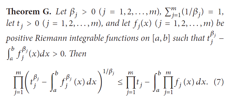
Aczel 不等式
\[ \begin{aligned} &a_i,b_i\in\mathbb{R},(i=1,2,\dots,n),\left(a_1^2>\sum_{i=2}^na_i^2\right)\text{ or }\left(b_1^2>\sum_{i=2}^nb_i^2\right)\\ \Rightarrow &\left(a_1^2-\sum_{i=2}^na_i^2\right)\left(b_1^2-\sum_{i=2}^nb_i^2\right)\le\left(a_1b_1-\sum_{i=2}^na_ib_i\right)^2 \end{aligned} \]
参数 B
- 在 \(r(x)\equiv\vert{g(x)}\vert\) 条件下找最优的 \(B\)
- 根据依据 \(1\)
\[ \begin{aligned} E[g(X)] &=\int \left(1-\dfrac{f(x)}{Bp(x)}\right)p(x)\;\mathrm{d}x\\ &=1-\dfrac{b}{B}\\ &=1-\dfrac{1}{\alpha B}\\ &=1-\dfrac{1}{BE[Y]}\\ \end{aligned} \]
- 得到
\[ \begin{aligned} \text{Eff} &=\dfrac{1}{c_0}\left(1-\int \vert{g(x)}\vert p(x)\;\mathrm{d}x\right)^2\\ &=\dfrac{\left(1-\int \vert{g(x)}\vert p(x)\;\mathrm{d}x\right)^2}{E\left[g^2(X)\right]E^2[Y]-\left(E\left[Y\right]-\dfrac{1}{B}\right)^2}\\ &=\dfrac{\left(1-E\left[\vert{g(X)}\vert\right]\right)^2}{E\left[g^2(X)\right]E^2[Y]-\left(E\left[Y\right]-\dfrac{1}{B}\right)^2}\\ (依据1)&=\dfrac{\left(1-E\left[\vert{g(X)}\vert\right]\right)^2}{E\left[g^2(X)\right]E^2[Y]-E^2\left[Y\right]E^2\left[g(X)\right]}\\ &=\dfrac{\left(1-E\left[\vert{g(X)}\vert\right]\right)^2}{V[g(X)]}\cdot\dfrac{1}{E^2[Y]}\\ \end{aligned} \]
- 再根据依据 \(2\)
\[ \begin{aligned} V[g(X)] &=V[g(X)-1]\\ &=V\left[-\dfrac{f(X)}{Bp(X)}\right]\\ &=\dfrac{1}{B}\cdot V\left[\dfrac{f(X)}{p(X)}\right]\\ \end{aligned} \]
- 于是
\[ \begin{aligned} \text{Eff} &=\dfrac{\left(1-E\left[\vert{g(X)}\vert\right]\right)^2}{V[g(X)]}\cdot\dfrac{1}{E^2[Y]}\\ &=\dfrac{\left(B-B\times E\left[\vert{g(X)}\vert\right]\right)^2}{V\left[\dfrac{f(X)}{p(X)}\right]}\cdot\dfrac{1}{E^2[Y]}\\ \end{aligned} \]
- 定义与 \(B\) 无关的量 \(c_1\)
\[ c_1=\dfrac{1}{V\left[\dfrac{f(X)}{p(X)}\right]\cdot E^2[Y]} \]
- 于是
\[ \begin{aligned} \text{Eff} &=c_1\cdot\left(B-B\times E\left[\vert{g(X)}\vert\right]\right)^2\\ &=c_1\cdot\left(B-\int\left\vert{B-\dfrac{f(x)}{p(x)}}\right\vert p(x)\;\mathrm{d}x\right)^2\\ &=c_1\cdot\left(\int\left(B-\left\vert{B-\dfrac{f(x)}{p(x)}}\right\vert\right) p(x)\;\mathrm{d}x\right)^2\\ &=c_1\cdot\left(\int f(x)\;\mathrm{d}x\right)^2\\ \end{aligned} \]
- 取等条件:\(B\ge\max\left\{\dfrac{f(x)}{p(x)}\right\}\)
几何分布
- 注意:在此条件下,RRS 没有分裂过程了
- \(r(x)=g(x)\in[0,1]\)
- 此时,随机变量 \(Y\) 退化如下
\[ Y=\dfrac{1}{B}+ \left\{ \begin{array}{rrl} Y,&\text{probability}&g(X)\\ 0,&\text{probability}&1-g(X)\\ \end{array} \right. \]
\[ \begin{aligned} &E[Y]=\dfrac{1}{B}+E[Y]\int g(x)p(x)\;\mathrm{d}x\\ \Rightarrow&E[Y]=\dfrac{1}{B(1-q)}\\ \end{aligned} \]
- 此时就是一个结果除以 \(B\) 的几何分布,继续概率 \(q=\int g(x)p(x)\;\mathrm{d}x\)
- 在此条件下,可以计算精确值
\[ C=\dfrac{1}{1-E[r(x)]}=\dfrac{1}{1-q} \]
\[ E[Y]=\dfrac{1}{B(1-q)} \]
\[ V[Y]=\dfrac{q}{B^2(1-q)^2}=qE^2[Y] \]
\[ \text{Eff}=\dfrac{1-q}{qE^2[Y]}=\left(\dfrac{1}{q}-1\right)\dfrac{1}{E^2[Y]} \]
- \(E[Y]\) 是 \(\alpha\) 的无偏估计,是常数
- 因此 \(q\) 越小越好,等价于 \(B\) 越小越好
\[ B=\max\left\{\dfrac{f(x)}{p(x)}\right\} \]