Ray Tracing-The Rest of Your Life(2)
Ray Tracing-The Rest of Your Life
4. Light Scattering
- 光线散射(反射、折射)
Albedo
- \(A\):albedo(whiteness 的拉丁语)
- 物体以概率 \(A\) 散射光线,以概率 \(1-A\) 吸收光线
- \(A\) 一般被定义为反射率,可以随着颜色、入射角的方向而变化
Scattering
- 很多基于物理的渲染器会使用一组不同波长的光表示光的颜色
- 我们之前使用的是 RGB,可以认为是一种对于长、中、短波的光的一种近似
- 我们实际看到的颜色就是如下的积分式子
\[ Color=\int A\cdot s(dir)\cdot\text{color}(dir) \]
- 这里的 dir表示的是 ray 的出射方向
- 因为光路是可逆的,我们使用从相机出发的 ray 效果是一样的
- \(s(dir)\) 表示朝着方向 dir
出射的概率
- \(s()\) 描述的就是一个出射方向的 pdf
- 当然,\(s()\)
可能和入射方向也有关,这样的话可以进一步描述为 \(s(view\_dir,dir)\)
- \(view\_dir\) 表示入射光的方向,也就是视线的方向
- \(\mathrm{color}(dir)\) 表示朝着 dir 这个方向的颜色,是递归定义
散射 pdf
- 利用 MC 框架进行计算
\[ Color=\dfrac{A\cdot s(dir)\cdot\text{color}(dir)}{p(dir)} \]
- \(p(dir)\) 是我们用于采样的 pdf
Lambertian 材质
\[ s(dir)=k\cos\theta \]
- \(\theta\) 表示出射方向 dir 和法线的夹角
- 我们是对立体角进行采样,等价于在球的表面进行采样,需要转化为 \(dS\)
- 法向半球采样
\[ \int k\cos\theta\;\mathrm{d}S =\int_{0}^{2\pi}\int_{0}^{\pi/2}k\cos\theta\sin\theta\;\mathrm{d}\theta\mathrm{d}\phi =k\pi=1 \]
- 于是有
\[ s(dir)=\dfrac{\cos\theta}{\pi} \]
- 我们可以使用和 \(s(dir)\)
相同的采样方式,\(p(dir)=s(dir)\)
- 这样子方差也不是为 0,方差为 0 的话应该是 \(p(dir)=s(dir)\cdot \mathrm{color}(dir)\)
- 还得归一化
- 这样子方差也不是为 0,方差为 0 的话应该是 \(p(dir)=s(dir)\cdot \mathrm{color}(dir)\)
- 于是我们得到
\[ Color=A\cdot\text{color}(dir) \]
- 这和我们之前得到的形式是一致的,但是我们需要泛化他,这样才能够结合新的采样方式
- 不一定是均匀采样,可能是对高贡献的方向多采样(例如导向光源)
- 文献中更多使用 BRDF 来描述
- Bidirectional Reflectance Distribution Function
- BRDF 定义如下
\[ BRDF=\dfrac{A\cdot s(dir)}{\cos\theta} \]
- 朗伯材质的表面散射的 BRDF 如下
\[ BRDF=\dfrac{A}{\pi} \]
- 也就是说
\[ Color=\dfrac{BRDF\cdot\cos\theta}{p(dir)}\cdot\text{color}(dir) \]
- 对于参与介质而言,通常称 albedo 为 scattering albedo,称 scattering
pdf 为 phase function
- participation media (volumes)
5. Importance Sampling Material
- 我们可以使用任意的 pdf 进行采样,任意的 pdf 都会让结果是无偏的,只是会影响收敛速度
- 我们期望我们结果的图片不要有太多噪点,希望采样到更多更亮的点
- 更多的向光源采样
- 我们记之前和 \(s()\) 相关的 pdf 为 \(\text{pSurface}(dir)\),和光源相关的 pdf 为 \(\text{pLight}(dir)\)
- 我们可以对这两种方式进行一个组合
- 如下是一个例子
\[ p(dir) = \frac{1}{2}\cdot \text{Light}(dir) + \frac{1}{2}\cdot \text{pSurface}(dir) \]
- 事实上,任意 \(0\le\alpha\le1\) 都是一个 pdf
\[ p(dir) = \alpha\cdot \text{Light}(dir) + (1-\alpha)\cdot \text{pSurface}(dir) \]
- 我们选择 pdf 的参考就是让 pdf 尽可能接近于 \(s(dir)\cdot\text{color}(dir)\)
- 简单地说,\(s(dir)\cdot\text{color}(dir)\) 越大的地方,我们期望 pdf 值越大
- 对于朗伯材质而言,一个猜测是,\(\text{color}(dir)\) 越大,pdf 越大
- 镜面材质,special case,出射方向比较小
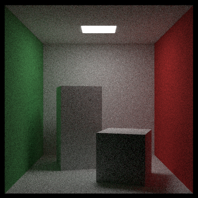
Cornell Box(1000spp)
- 以这个为例,开始降噪
- 166s
- 更新材质类,提供 pdf 功能
- Lambertian 余弦采样
- 171s

- 修改 pdf,法向半球采样
- 感觉噪点变重了,但是确实也是无偏的

6. 如何采样分布
- 简单化
- 将 \(z\) 轴作为法向量方向
- 只处理关于 \(z\) 轴旋转对称的情况
- 我们记 \(dir\) 和法向的夹角为 \(\theta\),此时有
\[ p(dir)=f(\theta) \]
- 我们指定一个分布 \(p(dir)=f(\theta)\)
- 我们都是认为在球面上采样
\[ \int f(\theta)\;\mathrm{d}S=1 \]
- 转化为 \(\theta,\phi\) 如下
\[ \int_{0}^{2\pi}\int_{0}^{\pi} f(\theta)\sin\theta\;\mathrm{d}\theta\mathrm{d}\phi=1 \]
- 我们能够得到边缘分布如下
\[ \begin{aligned} a(\phi) &=\int_{0}^{\pi} f(\theta)\sin\theta\;\mathrm{d}\theta\\ &=\dfrac{1}{2\pi}\int_{0}^{2\pi}\int_{0}^{\pi} f(\theta)\sin\theta\;\mathrm{d}\theta\mathrm{d}x\\ &=\dfrac{1}{2\pi}\\ \end{aligned} \]
\[ b(\theta)=\int_{0}^{2\pi}f(\theta)\sin\theta\;\mathrm{d}\phi=2\pi f(\theta)\sin\theta \]
- 我们指定 \(r_1,r_2\) 为满足 \([0,1]\) 均匀分布的随机变量,如何产生 \(\theta,\phi\) 呢?
- 利用之前的知识即可,cdf 相同或者直接求逆(单射)
球面均匀采样
\[ f(\theta)=\dfrac{1}{4\pi} \]
- 利用 cdf 相同,可以求得
\[ \phi=2\pi r_1 \]
\[ \begin{aligned} &\Pr(R_2\le r_2)=\Pr(\Theta\le\theta)\\ \Longrightarrow&\;r_2=\int_{0}^{\theta} 2\pi f(t)\sin t\;\mathrm{d}t=\dfrac{1-\cos\theta}{2}\\ \Longrightarrow&\;\cos\theta=1-2r_2\\ \end{aligned} \]
- 根据 \(x,y,z\) 变换
\[ \begin{array}{c} x = \cos(\phi) \cdot \sin(\theta)\\ y = \sin(\phi) \cdot \sin(\theta)\\ z = \cos(\theta)\\ \end{array} \]
- 得到
\[ \begin{array}{c} x = \cos(2\pi r_1) \cdot 2 \sqrt{r_2(1 - r_2)}\\ y = \sin(2\pi r_1) \cdot 2 \sqrt{r_2(1 - r_2)}\\ z = 1-2r_2\\ \end{array} \]
- 如此,我们得到了一个球面上的均匀采样
半球均匀采样
半球均匀采样
\[ f(\theta)=\dfrac{1}{2\pi} \]
- 类似的我们可以得到
\[ \phi=2\pi r_1,\cos\theta=1-r_2 \]
- 于是
\[ \begin{array}{c} x = \cos(2\pi r_1) \cdot \sqrt{r_2(2 - r_2)}\\ y = \sin(2\pi r_1) \cdot \sqrt{r_2(2 - r_2)}\\ z = 1-r_2\\ \end{array} \]
例子
- 一个半球采样的例子如下(朗伯反射)
\[ p(dir)=\dfrac{\cos\theta}{\pi} \]
- 计算
\[ r_2=\int_{0}^{\theta} 2\pi\dfrac{\cos t}{\pi}\sin t\;\mathrm{d}t=1-\cos^2\theta \]
\[ \phi=2\pi r_1 \]
- 变换
- 因为是半球,因此 \(z\ge0\)
\[ \begin{array}{c} x = \cos(2\pi r_1) \cdot \sqrt{r_2}\\ y = \sin(2\pi r_1) \cdot \sqrt{r_2}\\ z = \sqrt{1-r_2}\\ \end{array} \]
7. 正交基
- 正交基:orthonormal basis (ONB)
- 3 个正交向量
- 上面我们讨论了如何生成关于 \(z\)
轴旋转对称的分布,如何将其变换到关于法向对称分布?
- 坐标变换
- 我们使用的是简化版的坐标变换,只需要将 \(z\) 轴(局部坐标系)变换到法向(全局坐标系)即可
构建局部坐标系
- 有 \(\mathbf{n}\)(法线)
- 生成一个与 \(\mathbf{n}\)
不平行的方向 \(\mathbf{a}\)
- 判断 \(\mathbf{n}\) 是否为特定轴,如果不是则选取 \(\mathbf{a}\) 为某个轴即可
1 | if(n.x > 0.9): |
\[ \begin{array}{c} \mathbf{t}=\text{unit_vector}(\mathbf{a}\times \mathbf{n})\\ \mathbf{s}=\mathbf{t}\times \mathbf{n}\\ \end{array} \]
- 现在得到了标准正交基 \(\mathbf{s},\mathbf{t},\mathbf{n}\)
变换
- 标准正交基 \(\mathbf{s},\mathbf{t},\mathbf{n}\) 中方向坐标为 \((x,y,z)\)
- 全局坐标系中的方向为 \((x',y',z')\)
\[ \begin{pmatrix} \mathbf{s}^t\\\mathbf{t}^t\\\mathbf{n}^t\end{pmatrix} \begin{pmatrix} x'\\y'\\z' \end{pmatrix} = \begin{pmatrix} x\\y\\z \end{pmatrix} \]
- 于是
\[ \begin{pmatrix} x'\\y'\\z' \end{pmatrix} = \begin{pmatrix} \mathbf{s}^t\\\mathbf{t}^t\\\mathbf{n}^t\end{pmatrix}^t \begin{pmatrix} x\\y\\z \end{pmatrix} = \begin{pmatrix} \mathbf{s}&\mathbf{t}&\mathbf{n}\end{pmatrix} \begin{pmatrix} x\\y\\z \end{pmatrix} =x\mathbf{s}+y\mathbf{t}+z\mathbf{n} \]
- 此时利用上面说的方式采样,结果图如下
\[ p(dir)=\dfrac{\cos\theta}{\pi} \]

- 说实话看不出来很大区别