GAMES103.王华民.08.Finite Element Method II
有限元方法
- 方法
- The linear finite element method (FEM)
- The finite volume method (FVM)
- Hyperelastic models
FVM
- 有限体积方法
- Finite Volumn Method
- 对于四面体、三角形这种简单的、线性的 element 而言, 和之前的 FEM 方法是等价的
- 但是在推导和数学表示上,FVM 更清晰
- FEM 用能量对顶点位置求导得到力,FVM 对 traction vector 积分得到力
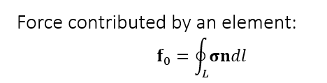
traction
- 考虑一个弹性体,被划分为上下两个部分
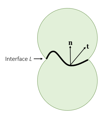
- 计算单位长度的力(traction)
- 3D:单位面积
- 那么合力就是积分
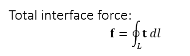
- 定义 stress tensor
- \(\sigma\)
- \(\mathbf{n}\):法向
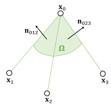
三角形
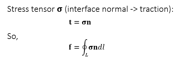
- 假设:一个顶点代表的不是一个点,而是一个区域
- 那么这个顶点受到的力就是外轮廓的积分
- 内力不对整体产生作用
- 绿色部分的力,绿色曲线上的积分
- 如何定义绿色曲线?
- 假设穿过边的中点
- 力对 3 个顶点的作用是平均的
- 中间无所谓
- 假设穿过边的中点
- stress 在三角形内部是均匀的(线性 element 假设),于是有
- 封闭曲线上的法向量积分等于 0
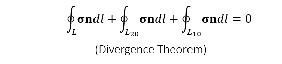
- 因此 \(L\) 上的力如下
- 直线上的法向相同
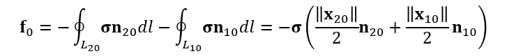
- 每个小三角形的 stress 不同,因此总的积分不为 0
3D
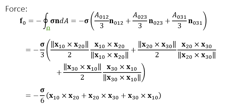
- 3 维的情况就是面积分
- 对 3 个表面的积分(下图没有画出背面)
- 计算如下
- 其中 \(\dfrac{1}{3}\) 也是想让面上的力对 3 个顶点的作用一样
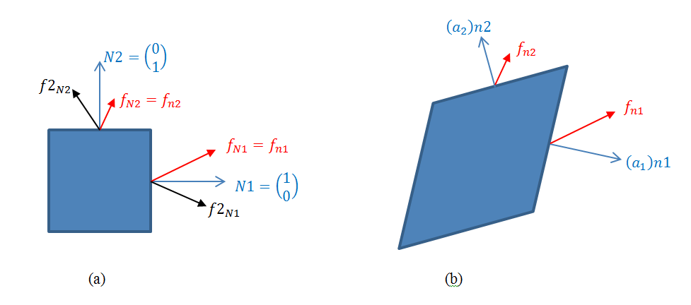
stress
- 如何计算 stress
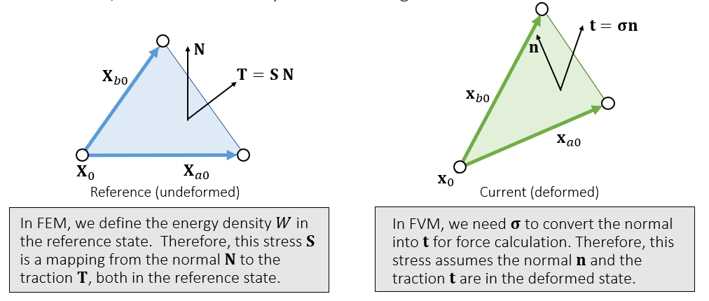
- 这里的 stress 是将 normal 映射到 traction 的一个矩阵
- FEM:stress 是定义在 reference 状态(没有形变)下的
- FVM:stress 是定义在 deformed 状态(有形变)下的
- 不同的 stress,根据 normal/traction 定义在没有形变/有形变的状态下分类
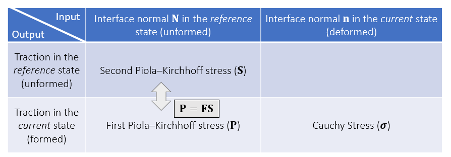
- 可以通过 \(\dfrac{\partial{W}}{\partial{G}}\) 求得 \(\mathbf{S}\)
- 通过 \(\mathbf{FS}\) 求得 \(\mathbf{P}\)
- \(\mathbf{P}=\mathbf{FS}\)
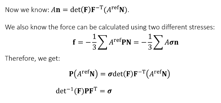
- 如何求得 \(\sigma\) ?
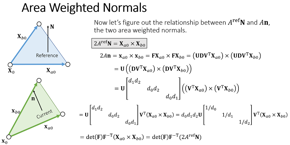
- 如何表示形变前后的 normal 之间的关系?
- 结论:\(\sigma=\det^{-1}(\mathbf{F})\mathbf{P}\mathbf{F}^{\mathbf{T}}\)
- \(\sigma=\det^{-1}(\mathbf{F})\mathbf{FS}\mathbf{F}^{\mathbf{T}}\)
- 推导如下
stress 关系
证明 1
- 如果 \(M\) 满足如下式子,那么有 \(\det(M)=\mathbf{a}\cdot(\mathbf{b}\times\mathbf{c})\)
\[ M=\det\begin{pmatrix}\mathbf{a}^\text{T}\\\mathbf{b}^\text{T}\\\mathbf{c}^\text{T}\end{pmatrix} =\det\begin{pmatrix}\mathbf{a}&\mathbf{b}&\mathbf{c}\end{pmatrix} \]
- 交换两行,行列式值改变符号
\[ \mathbf{a}\cdot(\mathbf{b}\times\mathbf{c}) =\mathbf{a}\cdot\det\begin{pmatrix}&\mathbf{b}^\text{T}&\\&\mathbf{c}^\text{T}&\\i&j&k\end{pmatrix} =\det\begin{pmatrix}\mathbf{b}^\text{T}\\\mathbf{c}^\text{T}\\\mathbf{a}^\text{T}\end{pmatrix} =\det\begin{pmatrix}\mathbf{a}^\text{T}\\\mathbf{b}^\text{T}\\\mathbf{c}^\text{T}\end{pmatrix} \]
证明 2
- Nanson’s Formula
- 如果矩阵 \(M\in\mathbb{R}^{3\times3}\) 可逆,而且 \(u,v\in\mathbb{R}^{3}\),那么有如下式子成立
\[ Mu\times Mv=\det(M)M^{-T}(u\times v) \]
- 设 \(w\) 是任意 \(\mathbb{R}^{3}\) 向量,于是有
\[ \begin{aligned} Mw\cdot(Mu\times Mv) &=\det\begin{pmatrix}Mw&Mu&Mv\end{pmatrix}\\ &=\det(M)\det\begin{pmatrix}w&u&v\end{pmatrix}\\ &=\det(M)\;w\cdot(u\times v) \end{aligned} \]
- 于是
\[ \begin{aligned} w\cdot\det(M)(u\times v) &=\det(M)\;w\cdot(u\times v)\\ &=Mw\cdot(Mu\times Mv)\\ &=w\cdot M^T(Mu\times Mv)\\ \end{aligned} \]
- 由于 \(w\) 的任意性,于是有
\[ M^{-T}(Mu\times Mv)=\det(M)(u\times v) \]
- 于是有
\[ Mu\times Mv=\det(M)M^{-T}(u\times v) \]
开始证明
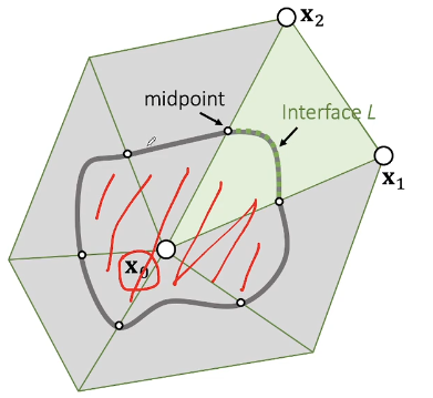
- 形变前/形变后
- 面积:\(A_{\text{ref}}/A\)
- 法线:\(A_\text{ref}\mathbf{N}/A\mathbf{n}\)
- 边:\(\mathbf{X}_{a0}/\mathbf{x}_{a0},\mathbf{X}_{b0}/\mathbf{x}_{b0}\)
- 根据不同 stress 的定义,我们有如下等式(都是计算形变后的受力)
\[ \mathbf{P}(A_{\text{ref}})\mathbf{N}=\sigma(A)\mathbf{n} \]
- 利用 Nanson’s Formula,可以得到
\[ \begin{aligned} (A)\mathbf{n} &=\dfrac{A}{\Vert\mathbf{x}_{a0}\times\mathbf{x}_{b0}\Vert_2}(\mathbf{x}_{a0}\times\mathbf{x}_{b0})\\ &=\dfrac{1}{2}(\mathbf{x}_{a0}\times\mathbf{x}_{b0})\\ &=\dfrac{1}{2}(\mathbf{F}\mathbf{X}_{a0}\times\mathbf{F}\mathbf{X}_{b0})\\ &=\dfrac{1}{2}\det(\mathbf{F})\mathbf{F}^{-\text{T}}(\mathbf{X}_{a0}\times\mathbf{X}_{b0})\\ &=(A_{\text{ref}})\det(\mathbf{F})\mathbf{F}^{-\text{T}}\mathbf{N}\\ \end{aligned} \]
- 类似的
\[ \begin{aligned} (A)\sigma\mathbf{n} &=\dfrac{A}{\Vert\mathbf{x}_{a0}\times\mathbf{x}_{b0}\Vert_2}\sigma(\mathbf{x}_{a0}\times\mathbf{x}_{b0})\\ &=\dfrac{1}{2}\sigma(\mathbf{x}_{a0}\times\mathbf{x}_{b0})\\ &=\dfrac{1}{2}\sigma(\mathbf{F}\mathbf{X}_{a0}\times\mathbf{F}\mathbf{X}_{b0})\\ &=\dfrac{1}{2}\sigma\det(\mathbf{F})\mathbf{F}^{-\text{T}}(\mathbf{X}_{a0}\times\mathbf{X}_{b0})\\ &=(A_{\text{ref}})\det(\mathbf{F})\sigma\mathbf{F}^{-\text{T}}\mathbf{N}\\ \end{aligned} \]
- 于是
\[ \begin{aligned} &(A_{\text{ref}})\mathbf{PN}=(A)\sigma\mathbf{n}\\ \Longrightarrow\;&\mathbf{P}=\det(\mathbf{F})\sigma\mathbf{F}^{-\text{T}}\\ \end{aligned} \]
- \(\mathbf{S}\) 的定义
\[ f2_{\mathbf{N}}=\mathbf{S}(A_{\text{ref}})\mathbf{N}=\mathbf{F}^{-1}f_{\mathbf{n}}=\mathbf{F}^{-1}\sigma(A)\mathbf{n} \]
- 如下图示,\(a\) 就表示 \(A_\text{ref}\)
- 定义:\(\mathbf{F}f2_{\mathbf{N}}=f_{\mathbf{n}}\)
- 根据
\[ \mathbf{S}(A_{\text{ref}})\mathbf{N}=\mathbf{F}^{-1}\sigma(A)\mathbf{n},(A_{\text{ref}})\mathbf{PN}=(A)\sigma\mathbf{n} \]
- 能够得到
\[ \mathbf{P}=\mathbf{FS} \]
\[ \mathbf{S}=\det(\mathbf{F})\mathbf{F}^{-1}\sigma\mathbf{F}^{-\text{T}} \]
重新表示力
- 第一行到第二行使用了两种不同的 stress 的表示方式
- 第一行:Cauchy Stress
- 第二行:First Piola–Kirchhoff stress
- 根据定义,两种表示都能计算得到力
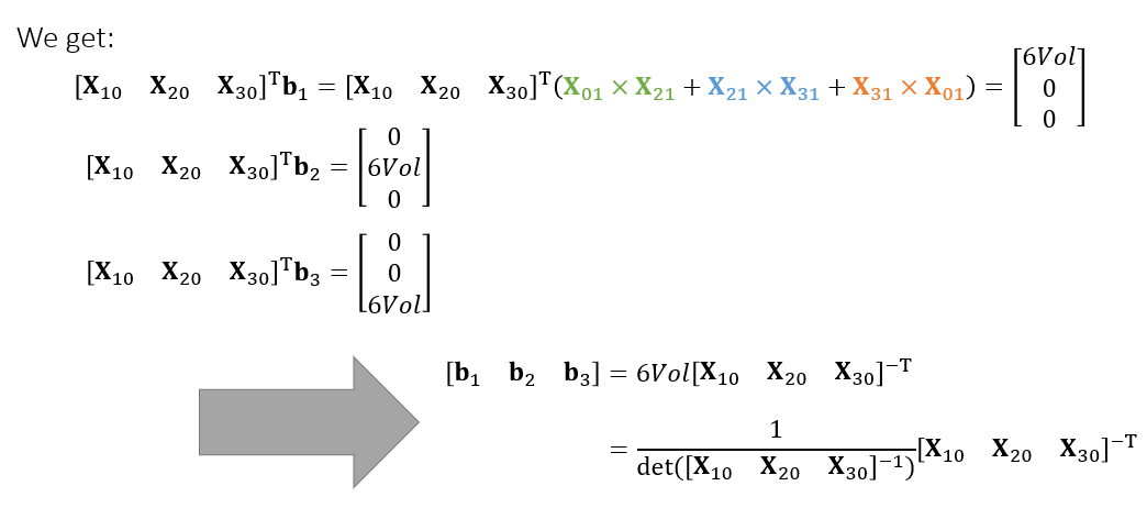
- \(\mathbf{b}_1\) 是简写
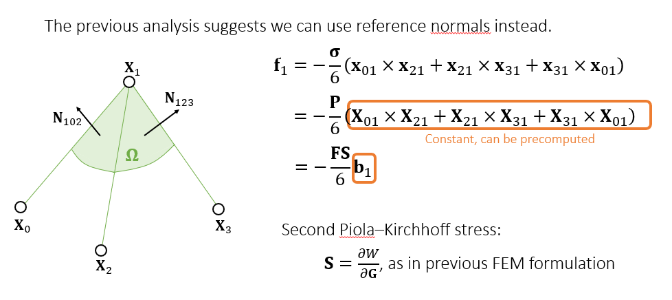
- \(\mathbf{b}_1\) 部分表示什么呢?
- 和三条边点乘
- 第二个式子:\(\mathbf{X}_{01}\times\mathbf{X}_{21}=\mathbf{X}_{01}\times(\mathbf{X}_{20}+\mathbf{X}_{01})=\mathbf{X}_{01}\times\mathbf{X}_{20}=\mathbf{X}_{20}\times\mathbf{X}_{10}\)
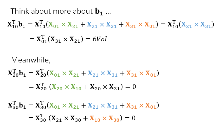
- 于是我们得到如下形式
代码框架
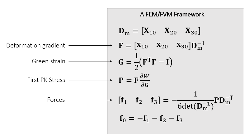
- 然后再用力去更新速度、更新位置
- FEM、FVM 在一般情况下是不一样的,但是在简单的 linear element 是一样的
论文
- Teran et al. 2003. Finite Volume Methods for the Simulation of Skeleton Muscles. SCA.
- Volino et al. 2009. A Simple Approach to Nonlinear Tensile Stiffness for Accurate Cloth Simulation. TOG.