(论文)[1997-SIG] Metropolis Light Transport(2)
Metropolis Light Transport
MLT
- 一些准备工作
- 将问题转化到 Metropolis 框架下
- 如何避免 start-up bias
- 设计高效的路径变异策略
Reduction to the Metropolis framework
- \(f_j(\bar{x})=w_j(\bar{x})f(\bar{x})\)
- \(w_j\):filter function,路径 \(\bar{x}\) 对像素 \(j\) 的贡献
- \(f\) 表示路径的贡献【和像素无关】
- \(w_j\) 只依赖于最后一条边 \(\mathrm{x}_{k-1}\mathrm{x}_k\),称为 lens edge
- MC 采样
\[ m_j=E\Big[\dfrac{1}{N}\sum_{i=1}^{N}\dfrac{w_j(\bar{X}_i)f(\bar{X}_i)}{p(\bar{X}_i)}\Big] \]
- 如果 \(p=\dfrac{1}{b}f\),那么
- \(b=\int_\Omega f(\bar{x})\;d\mu(\bar{x})\)
\[ m_j=E\Big[\dfrac{1}{N}\sum_{i=1}^{N}b\;w_j(\bar{X}_i)\Big] \]
- 此时 \(m_j\) 能被快速计算,因为一条光路一般只贡献给少量像素
- 问题:计算 \(b\),采样 \(p\propto f\)
- 采样问题可以使用 MLT 解决
- 但是 MLT 达到平衡,条件是 \(i\to\infty\)
- 实现上丢弃前 \(k\) 个样本(如何选取
\(k\) 很重要)
- start-up bias:如果选取的 \(k\) 太小,结果将很大程度上受到 \(\bar{X}_0\) 的影响
消除 start-up bias
- 思路上就是重采样,重采样后的分布更加接近 \(f(x)\) 本身
- 实现上就是重采样,然后求期望的时候自然就有一个 \(w\) 在采样概率中【加权】
- 初始路径 \(\bar{X}_0\)
通过容易的采样方式 \(p_0\)
采样得到【\(p_0\) 本身得是无偏的】
- 权重 \(W_0=\dfrac{f(\bar{X}_0)}{p_0(\bar{X}_0)}\)
- 此时 \(m_j\approx W_0w_j(\bar{X}_0)\)
- 接下来通过变异,依次得到 \(\bar{X}_1,\cdots,\bar{X}_N\)
- \(\bar{X}_i\) 有不同的分布 \(p_i\),只有当 \(i\to\infty\) 的时候,分布 \(p_i\propto\dfrac{1}{b}f\)
- 估计如下
\[ m_j=E\Big[\dfrac{1}{N}\sum_{i=1}^{N}w_j(\bar{X}_i){W_i}\Big]\tag{12} \]
- 我们将权重都设置为初始样本的权重 \(W_i=W_0\),此时结果是无偏的
- 下面讨论为什么这么设置是无偏的
无偏性证明
- 考虑 \(\bar{X}_0\) 是一组样本【无偏性基于此讨论】
- 如果 \(p_0=\dfrac{1}{b}f,W_0=b\),那么已经达到平衡,之后的分布
\(p_i=p_0\)
- \(W_i=\dfrac{f(\bar{X}_i)}{p_i(\bar{X}_i)}=b=W_0=\dfrac{f(\bar{X}_0)}{p_0(\bar{X}_0)}\)
- 于是 \(W_i=W_0=b\) 这样的设置是无偏的
- 对于一般的 \(p_0\),证明如下
- weighted equilibrium condition
- \(q_i\) 是第 \(i\) 个加权样本 \((W_i,\bar{X}_i)\) 的联合分布
- 表示重采样得到的第 \(i\) 个样本为 \(\bar{X}_i\),权重为 \(W_i\)
\[ \int_{\mathbf{R}}w\;q_i(w,\bar{x})\;\mathrm{d}w=f(\bar{x})\tag{16} \]
- 如果上面式子 \((16)\)
成立,那么无偏
- \(w_j(\cdot)\) 是 filter function,表示当前样本对像素 \(j\) 的贡献
\[ \begin{aligned} E\Big[w_j(\bar{X}_i){W_i}\Big]&=\int_{\Omega}\int_{\mathbf{R}}w\;w_j(\bar{x})\;q_i(w,\bar{x})\;\mathrm{d}w\;\mathrm{d}\mu(\bar{x})\\ &=\int_{\Omega}\;w_j(\bar{x})\;f(\bar{x})\;\mathrm{d}\mu(\bar{x})\\ &=m_j\\ \end{aligned} \]
- 式子 \((16)\) 对 \(q_0\) 是成立的
- \(q_0(w,\bar{x})=\delta(w-\dfrac{f(\bar{x})}{p_0(\bar{x})})p_0(\bar{x})\)
- \(\delta\):Dirac delta distribution
- 代入即得
- 而 \(W_0=\dfrac{f(\bar{X}_0)}{p_0(\bar{X}_0)}\) 就是设定
- \(q_0(w,\bar{x})=\delta(w-\dfrac{f(\bar{x})}{p_0(\bar{x})})p_0(\bar{x})\)
- 递推:因为设置了 \(W_i=W_{i-1}\)【也就是后续转移和 \(w\) 无关,\(w\) 只和初始样本有关】
\[ \begin{aligned} q_{i}(w,\bar{x})=&\Big[1-\int_{\Omega}T(\bar{y}|\bar{x})\;a(\bar{y}|\bar{x})\;\mathrm{d}\mu(\bar{y})\Big]q_{i-1}(w,\bar{x}) +\int_{\Omega}q_{i-1}(w,\bar{y})T(\bar{x}|\bar{y})\;a(\bar{x}|\bar{y})\;\mathrm{d}\mu(\bar{y})\\ &=q_{i-1}(w,\bar{x})+\int_{\Omega}\Big(-T(\bar{y}|\bar{x})\;a(\bar{y}|\bar{x})q_{i-1}(w,\bar{x}) +q_{i-1}(w,\bar{y})T(\bar{x}|\bar{y})\;a(\bar{x}|\bar{y})\Big)\;\mathrm{d}\mu(\bar{y})\\ \end{aligned}\ \]
- 于是乘上 \(w\),再积分;交换积分顺序【\(w\) 与后续样本无关】
\[ \begin{aligned} \int wq_{i}(w,\bar{x})\;\mathrm{d}w &=\int wq_{i-1}(w,\bar{x})\;\mathrm{d}w -\int\int_{\Omega}w\Big(T(\bar{y}|\bar{x})\;a(\bar{y}|\bar{x})q_{i-1}(w,\bar{x}) +q_{i-1}(w,\bar{y})T(\bar{x}|\bar{y})\;a(\bar{x}|\bar{y})\Big)\;\mathrm{d}\mu(\bar{y})\;\mathrm{d}w\\ &=f(\bar{x}) \int_{\Omega}\Big(-T(\bar{y}|\bar{x})\;a(\bar{y}|\bar{x})\left(\int wq_{i-1}(w,\bar{x})\;\mathrm{d}w\right) +\left(\int wq_{i-1}(w,\bar{y})\;\mathrm{d}w\right)T(\bar{x}|\bar{y})\;a(\bar{x}|\bar{y})\Big)\;\mathrm{d}\mu(\bar{y})\\ &=f(\bar{x}) +\int_{\Omega}\Big(-T(\bar{y}|\bar{x})\;a(\bar{y}|\bar{x}) f(\bar{x}) + f(\bar{x})T(\bar{x}|\bar{y})\;a(\bar{x}|\bar{y})\Big)\;\mathrm{d}\mu(\bar{y})\\ \end{aligned} \]
- 根据细致平衡条件,于是成立
- 注意这里是 \(f\),所以一直满足
Initialization
- 初始化 \(X_0\) 为一个样本效果不好
- \(W_0\) 很可能为 0,导致初始阶段值都为 0
- 跑 \(n\) 个并行算法
- 我们实现
- 采样大量路径 \(\bar{X}^{(i)}_0\),记录他们的权重 \(W_0^{(1)}\)
- 重采样获取 \(n'\) 个
equal-weighted paths
- chosen with equal spacing in the cumulative weight distribution of the \(\bar{X}_0^{(i)}\)
- 作为 MLT 的独立的随机种子
- 通常我们选择 \(n'=1\)
- 初始化的目的是算一个 \(W_0\) 的均值
- 实际测试中,初始化这一步的开销很小
- two phase
- 初始化估计平均亮度
- 之后估计每个像素的相对亮度
Convergence tests
- 需要跑多个种子 \(n'>1\),因为一次生成的样本相关性高
Spectral sampling
- 光谱采样,就能将 color 转化为 scalar
- image contribution function \(f\) 对选定波长计算
- 波长重要性采样:\(h/p\),\(p\) 正比于 luminance
设计变异策略
MLT 的问题:样本存在相关性,引入高方差
- 原因:拒绝太多;变异太小
一些 mutation 需要具备的特征
- High acceptance probability
- 低接受率导致有很多样本都一样,全在一个像素上,显示为噪声
- Large changes to the path
- 小的变化还是会导致高相关性
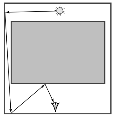
- Ergodicity【遍历】
- 陷入一个局部的路径子空间出不来,导致积分值小于 \(b\)(相当于不能覆盖整个定义域,有偏了)
- 要求任意两个有贡献的路径互相可达
- 例如下图,如果只允许增删点,那么不能变换到右边可行路径【变异策略不行】
- Changes to the image location
- 希望修改 lens edge \(\mathrm{x}_{k-1}\mathrm{x}_{k}\),我们希望估计 \(f\)
- 也就是希望估计 \(f\) 在像素平面的分布,所以希望改位置
- Stratification
- 不够平均
- "balls in bins" effect:\(n\) 球选 \(n\) 桶,很难恰好平均分配
- Low cost
- High acceptance probability
好的变异策略
- 3 种策略
- bidirectional mutations
- perturbations
- lens subpath mutations
- 有些细节结合这个教程看
Bidirectional mutations
思路:替换当前路径 \(\bar{x}=\mathrm{x}_0\cdots\mathrm{x}_k\) 中的部分子路径
\(p_{\text{d}}[s,t]\) 概率删除子路径 \(\mathrm{x}_s\cdots\mathrm{x}_t\)【不包括端点】
- \(-1\le s<t\le k+1\)
两个因子相乘
- \(p_{\text{d},1}\):倾向于删除短路径【成本低,接受度高】
- \(p_{\text{d},2}\):接受度高【见章节 refinemnents】
新路径:希望和旧路径相似【接受度高】
两步:\(p_{\text{a}}[s',t']=p_{\text{a},1}p_{\text{a},2}\)
- 先选长度 \(l_{\text{a}}=s'+t+1\),倾向于保持不变【离散分布 \(p_{\text{a},1}\)】
- 选择 \(s',t'\)【离散分布 \(p_{\text{a},2}\),均匀选 \(s'\)】
选取节点:BSDF 采样【如果是空路径则在光源/相机上均匀选点】
- 找到之后连起来
- 拒绝:不可见;打空
有概率删除整条路径【为了保证遍历性】
参数设定
\[ p_{\text{d},1}[l_{\text{d}}]= \left\{ \begin{array}{ll} 0.25,&l_{\text{d}}=1\\ 0.5,&l_{\text{d}}=2\\ 2^{-l_{\text{d}}},&l_{\text{d}}\ge3\\ \end{array} \right. \]
\[ p_{\text{a},1}[l_{\text{a}}]= \left\{ \begin{array}{ll} 0.5,&l_{\text{a}}=l_{\text{d}}\\ 0.15,&l_{\text{a}}=l_{\text{d}}-1\\ 0.15,&l_{\text{a}}=l_{\text{d}}+1\\ &\text{other possible lengths}\\ \end{array} \right. \]
- 接收率:\(a(\bar{y}|\bar{x})=\dfrac{f(\bar{y})T(\bar{x}|\bar{y})}{f(\bar{x})T(\bar{y}|\bar{x})}=\dfrac{R(\bar{y}|\bar{x})}{R(\bar{x}|\bar{y})}\)
- \(R(\bar{y}|\bar{x})=\dfrac{f(\bar{x})}{T(\bar{y}|\bar{x})}\)
- 需要考虑多种可能的生成方式,一条路径可能有多种生成方式
例子 1
- \(\mathbf{x}_0\mathbf{x}_1\mathbf{x}_2\mathbf{x}_3\) 变成 \(\mathbf{x}_0\mathbf{x}_1\mathbf{z}_0\mathbf{x}_2\mathbf{x}_3\),对应选择为 \((s,t,s',t')=(1,2,1,0)\)
- 忽略 \(f\) 分子分母相同项
\[ f(\bar{y})=f_{\text{s}}(\mathbf{x}_0,\mathbf{x}_1,\mathbf{z}_0)G(\mathbf{x}_1,\mathbf{z}_0)f_{\text{s}}(\mathbf{x}_1,\mathbf{z}_0,\mathbf{x}_2)G(\mathbf{z}_0,\mathbf{x}_2)f_{\text{s}}(\mathbf{z}_0,\mathbf{x}_2,\mathbf{x}_3) \]
\[ T(\bar{y}|\bar{x})=p_{\text{d}}[1,2]\Bigg[ p_{\text{a}}[1,0] p_{\text{s}}(\mathbf{x}_0,\mathbf{x}_1,\mathbf{z}_0) G(\mathbf{x}_1,\mathbf{z}_0) + p_{\text{a}}[0,1] p_{\text{s}}(\mathbf{x}_3,\mathbf{x}_2,\mathbf{z}_0) G(\mathbf{x}_2,\mathbf{z}_0)\Bigg] \]
- 另外 \(R(\bar{x}|\bar{y})\) 如下
- 这里的 \(p\) 是基于路径 \(\bar{y}\) 计算的
\[ \left\{f_{\text{s}}(\mathbf{x}_0,\mathbf{x}_1,\mathbf{x}_2)G(\mathbf{x}_1,\mathbf{x}_2)f_{\text{s}}(\mathbf{x}_1,\mathbf{x}_2,\mathbf{x}_3)\right\}\Bigg/\left\{p_{\text{d}}[1,3]p_{\text{a}}[0,0]\right\} \]
- 预计算
\[ \begin{aligned} C(\mathbf{x}_0,\mathbf{x}_1,\mathbf{x}_2,\mathbf{x}_3) &= f_{\text{s}}(\mathbf{x}_0,\mathbf{x}_1,\mathbf{x}_2)G(\mathbf{x}_1,\mathbf{x}_2)f_{\text{s}}(\mathbf{x}_1,\mathbf{x}_2,\mathbf{x}_3)\\ S(\mathbf{x}_0,\mathbf{x}_1,\mathbf{x}_2) &= f_{\text{s}}(\mathbf{x}_0,\mathbf{x}_1,\mathbf{x}_2)/p_{\text{s}}(\mathbf{x}_0,\mathbf{x}_1,\mathbf{x}_2) \end{aligned}\tag{14} \]
- 这里需要考虑 \(\mathbf{x}_0\mathbf{x}_1\mathbf{x}_2\mathbf{x}_3\to\mathbf{x}_0\mathbf{x}_3\to\mathbf{x}_0\mathbf{x}_1\mathbf{z}_0\mathbf{x}_2\mathbf{x}_3\)
这样的情况吗?
- 【论文是不考虑的,算的话太复杂了,不太懂】
Perturbations
- 处理这样的情况:局部贡献值很大
- 焦散,穿过小孔,concave corners where two surfaces meet
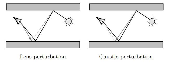
Lens perturbations
- 删除 \((L|D)DS^{\ast}E\) 形式的路径
- lens subpath做扰动
- 随机距离 \(R\),随机角度 \(\phi\)(均匀)
- \(\xi\sim \mathcal{U}[0,1]\)
\[ R=r_2\exp(-\ln(r_2/r_1)\xi),r_1<r_2 \]
- 经过相同的 specular 次数(保留反射/折射模式),然后连原始路径
Caustic perturbations
- \(LS^{+}DE\) 路径
- 删除 \((D|L)S^{\ast}DE\) 形式路径
- 扰动 diffuse 表面
- \(\theta\) 指数分布,\(\phi\) 均匀分布
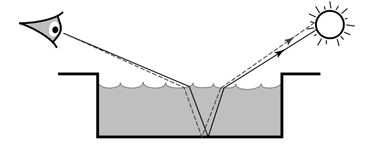
Multi-chain perturbations
- \((D|L)DS^{\ast}DS^{\ast}DE\)
- 水中焦散,是这个光路吗?
- 在每一个 non-specular 的点,做出射方向的扰动
参数设置
- \(r_1=0.1 \text{ pixels}\)。\(r_2\) 使得扰动区域占图片的 5%
- \(\theta_1=0.0001\text{ radian}\),\(\theta_2=0.1\text{ radian}\)
Lens subpath mutations
- lens subpath 光路类型 \((L|D)S^{\ast}E\)
- 初始化构建 \(n'\)
条独立的种子路径
- which are mutated in a rotating sequence
- 任意时刻我们保存 current lens subpath \(\bar{x}_{\text{e}}\)
- eye subpath mutation 包括删除 lens subpath 然后替换成 \(\bar{x}_{\text{e}}\)
- \(\bar{x}_{\text{e}}\) 被重用 \(n_{\text{e}}\) 次之后,生成新的(\(n'\gg n_{\text{e}}\)),避免在同样路径上多次重复使用相同的 lens subpath
- 生成 \(\bar{x}_{\text{e}}\):图像平面选择一个点,发射光线,弹弹弹,知道遇到
non-specular 顶点
- 通过记录像素已经生成了多少条 subpath,使得新生成的 subpath
在全局比较平均
- We use a rover to make the search for a non-full pixel efficient【优化查找还有空余配额的像素】
- 像素内部样本分布
- Poisson minimum-disc pattern
- 通过记录像素已经生成了多少条 subpath,使得新生成的 subpath
在全局比较平均
选择突变类别
- 平衡选择 3 种策略
- 因为不同策略对应不同光路,我们很难提前知道哪种策略好
Refinements
- 提高效率
- Direct lighting:直接做就很高效
- 直接光不用 MLT
- Using the expected sample value
- 原来是 \(a(\bar{y}|\bar{x})\) 概率累计 \(\bar{x}\),\(1-a(\bar{y}|\bar{x})\) 概率累计 \(\bar{y}\)
- 改成直接都累计,累积量:\(a(\bar{y}|\bar{x})\bar{x}+(1-a(\bar{y}|\bar{x}))\bar{y}\)
- 理解推导
- 突变概率的重要性采样
- 给定删除的 subpath \(\mathrm{x}_s\cdots\mathrm{x}_t\)
- 可以计算接收率的一些因子
- \(a(\bar{y}|\bar{x})\propto 1/R(\bar{x}|\bar{y})\),\(R\) 的分子可以计算,将其作为 \(p_{\text{d},2}\)
- \(p_{\text{d},2}[1,2]=1/C(\mathbf{x}_0,\mathbf{x}_1,\mathbf{x}_2,\mathbf{x}_3)\)
- 根据这个权重,选择变异策略
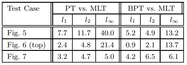
Results
- MLT、PT、BDPT
- MLT 效果显著好,焦散处理好
- 一般场景下:MLT 亮处好,BDPT 暗处好
- 同时间对比,计算 \(e_j=(\tilde{m}_j-m_j)/m_j\),然后计算他们的范数
- 表格里面是除以 MLT 的结果